25 years ago

In 1998 I published the 1st issue of the Excel Experts ELetter. EEE was intended to share the cutting edge Excel tips and tricks with the Excel developers of the world. 21 issues were published. Surprisingly, much of the content is still relevant today. A file containing an archive of this information is available on this website.

LAMBDA EXCEL: DUPONT ROE

As I mentioned in a previous article on the implementation of the new LAMBDA function in Excel, it was targeted (IMO) at commonly used but very complex Excel formulas and calculations. I became acquainted with one such formula while reading about it on LinkedIn in a discussion about accounting, which I have to admit is not one of my favorite subjects. Thus, I had never heard of the Dupont analysis formula. After reading about it, I thought it was a perfect candidate for the LAMBDA treatment. The details on how it was constructed and how it can be used can be found at:

wallstreetprep.com/knowledge/dupont-analysis-template/

There is the 3-point and the 5-point flavor of this calculation, and I chose the 5-point. The inputs used for this calculation can be viewed in the following figure.

So, to make a LAMBDA formula for this that can be entered as

=DuPontROE(B5,B6,B7,B8,B9,B10)

you would use define the following formula in Name Manager as DupontROE:

=LAMBDA(Assets,Equity,Sales,EBIT,EBT,Net_income,LET(Margin,EBIT/Sales,Turnover,Sales/Assets,Cost_Ratio,EBT/EBIT,Equity_Multiplier,Assets/Equity,Tax_effect_ratio,Net_income/EBT,Margin*Turnover*Cost_Ratio*Equity_Multiplier*Tax_effect_ratio))

This is just one example of what must be a lot of exciting Excel accounting formulas out there in the world, just waiting to be converted to a useful and easily useable Excel LAMBDA formula. If you are an Excel accounting guru, it is time to start doing this!

LAMBDA EXCEL: WtFrac (percentage of an element in a chemical compound)

The calculation of molecular weight using LAMBDA can be seen in the link below.

The algorithm used to return molecular weight with an Excel formula was developed by ExcelXOR based on a challenge I gave him. It was amazing!

But it was not designed to be used in further calculations and it took a while (years?) before I figured out a way to use it to get other molecular information. In particular, it would be useful to calculate the weight fraction of a specified atomic unit in a given molecule.

For example, the ability to calculate the weight fraction of “Ca” in the molecule “Ca3(PO4)2” using only Excel formulas would be powerful. When Microsoft released the LET and LAMBDA functions, it provided a way to accomplsh this.

Define WtFrac as:

=LAMBDA(at,molec,

LET(s,SEQUENCE(LEN(molec)),

arr,IFERROR(INDEX(AWeight,MATCH(MID(molec,s,MMULT(0+(ABS({77.5,107.5}-CODE(MID(MID(molec&”ζ”,s,2),{1,2},1)))<13),{1;1})),Atom,0)),0)IFERROR(0+MID(molec,MMULT(0+(ABS({77.5,107.5}-CODE(MID(MID(molec&”ζ”,s,2),{1,2},1)))<13),{1;1})+s,MMULT(1-ISERR(0+MID(molec,s+MMULT(0+(ABS({77.5,107.5}-CODE(MID(MID(molec&”ζ”,s,2),{1,2},1)))<13),{1;1}),{1,2})),{1;1})),1)IFERROR(0+MID(molec,IF(ISNUMBER(MATCH(s,IF(ISODD(MATCH(s,MODE.MULT(IF(MID(molec,s,1)={“(“,”)”},s+{1,0}),s))),s),0)),FIND(“)”,molec,s))+1,MMULT(1-ISERR(0+MID(molec,IF(ISNUMBER(MATCH(s,IF(ISODD(MATCH(s,MODE.MULT(IF(MID(molec,s,1)={“(“,”)”},s+{1,0}),s))),s),0)),FIND(“)”,molec,s))+1,{1,2})),{1;1})),1)/MW(at),

SUM(IF(arr=INT(arr),arr,0)))*MW(at)/MW(molec))

Using the WtFrac formula, =WtFrac(“Ca”,”Ca3(PO4)2″) affords a value of 0.38763, or, stating differently, the amount of calcium in calcium phosphate is 38.763 %.

Using this formula, more complex mixtures of chemical compounds can be calculated. Time and health permitting, maybe you will see this as my next LAMBDA project.

LAMBDA EXCEL: Simple Moving Average

by David Hager

Just for fun: What is the hottest pork BBQ sauce? Give answers in comments and I will give mine in a subsequent post.

Although I cannot read Microsoft’s mind, I am fairly certain that the LAMBDA function was created to convert complex and commonly used worksheet formulas into named formulas that can be used by a normal Excel user without having to copy/paste those large formulas. Since there are literally millions of successfully used formulas in Excel applications that cannot be accessed for this type of conversion until companies upgrade their Office versions (i.e. – 365), those in the Excel community either have to create new (and incredibly powerful) Lambdas or convert formulas that are globally available.

In this latter category, virtually all manner of charting data uses different types of moving averages. The most basic form of moving average is commonly referred to as the simple moving average. Briefly, in a column of data the first n rows can be averaged to afford a single data point, which would be the first point in the new series. For example, in A1:A10, the first point in column B would be AVERAGE (A1:A10) in cell B10. This formula can be copied down for subsequent points. However, the goal would be to have a single formula for ALL moving averages. If A1:A25 contained the data and an 8 point moving average was desired, the formula =SMA(arr,n) starting in B1 would return the desired result. Since formulas in B1:B7 would be trying to return a result with less than 8 data points, an error would occur and, for charting purposes, NA() would be returned for those cells. The LAMBDA formula that would fit these requirements is:

=LAMBDA(arr,n,LET(x,SCAN(0,arr,LAMBDA(x,y,x+1)),IF(x>=n,AVERAGE(INDEX(arr,x-n+1):INDEX(arr,x)),NA())))

The key part of this formula is SCAN(0,arr,LAMBDA(x,y,x+1)), which basically counts each row in the array. Thus, for every “event” that occurs, the value of x can be used for whatever mathematical operation is needed (in this case, AVERAGE).

Hopefully, there will be new LAMBDA blog posts coming soon!

LAMBDA EXCEL: DewPoint

Well, I had been waiting for Microsoft to release the LAMBDA (and helper) functions to the general public since my last post (over a year ago) so I decided to stop waiting and create another post. Just as a reminder, most large companies have created complex formulas to calculate proprietary information and the people who made these formulas have likely not documented how they work and they have either passed (literally or moved on to another company) or they will do so soon. So, virtually any formula that requires inputs (and some that don’t – see my LAMBDA article on this blog on the BINGO function) can be converted into a LAMBDA formula. The two main advantages of this is that they are self-documenting and the complex logic used in the formula is hidden away in defined names. In this example, a formula that calculates the dew point will be converted into a LAMBDA formula.

There are a number of formulas that have been made that use temperature (°F in this example) and relative humidity as inputs to return the dewpoint. They contain constants that were derived from curve fitting based on data. The following formula is one example of this (original author is unknown).

(243.04*(LN(h/100)+((17.625*t)/(243.04+t))))/(17.625-(LN(h/100)+( (17.625*t)/(243.04+t))))

where t is temperature and h is relative humidity.

The corresponding LAMBDA formula for this is

=LAMBDA(t,h,(243.04*(LN(h/100)+((17.625*t)/(243.04+t))))/(17.625-(LN(h/100)+( (17.625*t)/(243.04+t)))))

and when entered into the Name Manager with the name “Dewpoint”

the new formula can be entered into a worksheet cell as

=Dewpoint(85,60) which return a value of 72.65°F.

If a value for h<0 issued, the expected error value will be returned since negative humidity is not possible. However, if h>100, the native formula still returns a result, although incorrect since the humidity cannot be greater than 100. Thus, the LAMBDA formula can be amended as shown below.

=LAMBDA(t,h,IF(h>100,NA(),(243.04(LN(h/100)+((17.625t)/(243.04+t))))/(17.625-(LN(h/100)+( (17.625*t)/(243.04+t))))))

Be watching here on this blog for more LAMBDA excitement!

LAMBDA EXCEL: Letter Grade

BY DAVID HAGER In a continuing series of posts on showing how to convert (long, but not necessarily long) Excel formulas into lambda functions, here is an useful formula I created for use in applying letter grades to numeric scores. #Excel Short and Sweet Tip #17 (Returning a Letter Grade Based on a Normal Grading Scale Without Lookup Table) by David Hager | Excel For You (wordpress.com) This formula is shown below. The “letter buckets” that correspond to each grade might not fit all situations. =IF(A5>=90,”A”,IF(A5>=80,”B”,IF(A5>=70,”C”,IF(A5>=60,”D”,”F”))))&IF(A5>98,”+”,IF(A5<59,””,IF(OR(RIGHT(A5,1)={“1″,”2″,”0″}),”-“,IF(OR(RIGHT(A5,1)={“8″,”9″}),”+”,””)))) In the Name Manager, assign a new name of LetterGrade. In the Refers To box, place the lambda form of the letter grade formula: =LAMBDA(grade,IF(grade>=90,”A”,IF(grade>=80,”B”,IF(grade>=70,”C”,IF(grade>=60,”D”,”F”))))&IF(grade>98,”+”,IF(grade<59,””,IF(OR(RIGHT(grade,1)={“1″,”2″,”0″}),”-“,IF(OR(RIGHT(grade,1)={“8″,”9″}),”+”,””))))) Then, if =LetterGrade(88) was placed in a cell, the result would be “B+”. Currently, only those users of Excel 365 that are in the Office Insiders beta program have access to the LAMBDA function. However, it is not too early to start collecting your favorite converted formulas so you will be ready to use them when it is available to you.

LAMBDA EXCEL: Bible Verse

BY DAVID HAGER

One of my first blog posts about the use of Excel’s web functions was about a method to return a specified Bible verse.

Lookup a Bible Verse Using #Excel (w/o VBA) by David Hager – Excel For You (wordpress.com)

It used several lookup techniques involving Excel data validation lists from worksheet cells to allow the user to select the desired verses. However, I decided to use retrieving a Bible verse using the new LAMBDA conversion, which required using a different way to get the information directly from the Bible verse. Thus, I needed to create some string manipulation formulas to use in the master formula. The new methodology can be seen in the formula below.

If BVerse = 1 Samuel 2:13 then

=FILTERXML(WEBSERVICE(“http://labs.bible.org/api/?passage=”&amp;

LEFT(BVerse,LOOKUP(2^15,FIND(” “,BVerse,SEQUENCE(LEN(BVerse))))-1)&” “&

MID(BVerse,LOOKUP(2^15,FIND(” “,BVerse,SEQUENCE(LEN(BVerse))))+1,FIND(“:”,BVerse)-LOOKUP(2^15,FIND(” “,BVerse,SEQUENCE(LEN(BVerse))))-1)&”:”&MID(BVerse,FIND(“:”,BVerse)+1,255)

&”&type=xml”),”//text”)

where the book of the bible verse is

=LEFT(BVerse,LOOKUP(2^15,FIND(” “,BVerse,SEQUENCE(LEN(BVerse))))-1)

and the chapter of the bible verse is

=MID(BVerse,LOOKUP(2^15,FIND(” “,BVerse,SEQUENCE(LEN(BVerse))))+1,FIND(“:”,BVerse)-LOOKUP(2^15,FIND(” “,BVerse,SEQUENCE(LEN(BVerse))))-1)

and the verse number is

=MID(BVerse,FIND(“:”,BVerse)+1,255)

So, then 1 Samuel is the book, 2 is the chapter and 13 is the verse number.

To convert this into a LAMBDA formula, in the Name Manager the new name should be BibleVerse and in the Refers To box should be written:

=LAMBDA(BVerse,FILTERXML(WEBSERVICE(“http://labs.bible.org/api/?passage=”&LEFT(BVerse,LOOKUP(2^15,FIND(” “,BVerse,SEQUENCE(LEN(BVerse))))-1)&” “&MID(BVerse,LOOKUP(2^15,FIND(” “,BVerse,SEQUENCE(LEN(BVerse))))+1,FIND(“:”,BVerse)-LOOKUP(2^15,FIND(” “,BVerse,SEQUENCE(LEN(BVerse))))-1)&”:”&MID(BVerse,FIND(“:”,BVerse)+1,255)&”&type=xml”),”//text”))

(Based on the naming convention used in the xml source, if the first part of the book name has a number like 1st, 2nd or 3rd, the bible verse string should always be written with a 1, 2, or 3.)

Thus, again for 1 Samuel 2:13 in A1, if =BibleVerse(A1) is typed in B1, the return value is:

“This was the priests’ routine with the people. Whenever anyone was making a sacrifice, the priest’s attendant would come with a three-pronged fork in his hand, just as the meat was boiling.”

An Excel file containing the described LAMBDA function can be downloaded by clicking the following link.:

BTW, if the Bible verse is written incorrectly, the IFERROR function can be used to encapsulate the LAMBDA formula to return a Not Found message if desired.

Stay tuned for more great LAMBDA Excel creations!

LAMBDA Excel: BINGO

BY DAVID HAGER Here’s a quick and interesting use of the LAMBDA function as an adieu to 2020. I have written several blog posts on the creation of a Bingo board; the latest can be found here: Excel #8 – Making a Bingo Card Using Only Formulas with Dynamic Array Functions | Excel For You (wordpress.com) I realized that this would provide a good example of LAMBDA without any variables. So, in the Excel Name Manager, create a new name called BINGO. In the Refers To box, copy/paste this formula and click Close. =LAMBDA(INDEX(SORTBY(SEQUENCE(15),RANDARRAY(15))+(15*(SEQUENCE(,5)-1)),SEQUENCE(5),SEQUENCE(,5))) Then, enter =BINGO() in any cell. This one formula will return a 5 X 5 range of unique numbers that correspond to the 5 columns of a Bingo card. The only actions left are to add the B I N G O column headers and format the central cell with a black fill. Happy New Years, and continue watching for additional LAMBDA creations.

LAMBDA Excel: Molecular Weight

BY DAVID HAGER This is my first post of many to come about the Excel LAMBDA function. Shown below are the first and best videos about LAMBDA.

I strongly recommend that you watch these videos so that you will truly appreciate how LAMBDA will supercharge the Excel spreasheet. In this and subsequent posts, I will be looking at complex Excel formulas that I and others have made and demonstrating how they can be converted to reusable Excel functions with LAMBDA. So, I might as well start with the most complex Excel formula ever made. At my request, the creator of the EXCELXOR blog made an Excel formula that calculates the molecular weight from a chemical formula string. It works, but the creator would take a LONG time to explain how it works. Feel free to study it at the link shown below if you have a few weeks to kill. Molecular Weights « EXCELXOR I have modified the original formula slightly to make it amenable for conversion to a LAMBDA function, and you could study this formula as well, but simply trust me that this is exactly the situation LAMBDA was made for and you can use it if you need to. =LAMBDA(molecule,SUM(IFERROR(INDEX(AWeight,MATCH(MID(molecule,SEQUENCE(LEN(molecule)),MMULT(0+(ABS({77.5,107.5}-CODE(MID(MID(molecule&"ζ",SEQUENCE(LEN(molecule)),2),{1,2},1)))<13),{1;1})),Atom,0)),0)IFERROR(0+MID(molecule,MMULT(0+(ABS({77.5,107.5}-CODE(MID(MID(molecule&"ζ",SEQUENCE(LEN(molecule)),2),{1,2},1)))<13),{1;1})+SEQUENCE(LEN(molecule)),MMULT(1-ISERR(0+MID(molecule,SEQUENCE(LEN(molecule))+MMULT(0+(ABS({77.5,107.5}-CODE(MID(MID(molecule&"ζ",SEQUENCE(LEN(molecule)),2),{1,2},1)))<13),{1;1}),{1,2})),{1;1})),1)IFERROR(0+MID(molecule,IF(ISNUMBER(MATCH(SEQUENCE(LEN(molecule)),IF(ISODD(MATCH(SEQUENCE(LEN(molecule)),MODE.MULT(IF(MID(molecule,SEQUENCE(LEN(molecule)),1)={"(",")"},SEQUENCE(LEN(molecule))+{1,0}),SEQUENCE(LEN(molecule))))),SEQUENCE(LEN(molecule))),0)),FIND(")",molecule,SEQUENCE(LEN(molecule))))+1,MMULT(1-ISERR(0+MID(molecule,IF(ISNUMBER(MATCH(SEQUENCE(LEN(molecule)),IF(ISODD(MATCH(SEQUENCE(LEN(molecule)),MODE.MULT(IF(MID(molecule,SEQUENCE(LEN(molecule)),1)={"(",")"},SEQUENCE(LEN(molecule))+{1,0}),SEQUENCE(LEN(molecule))))),SEQUENCE(LEN(molecule))),0)),FIND(")",molecule,SEQUENCE(LEN(molecule))))+1,{1,2})),{1;1})),1))) or, =MolecularWeight(A1), whichever is easier 😁. There are parts of this formula that could be simplified by using the LET function, so if you would like to do this, feel free, but 99% of users that would not gain any readability. What is important is understanding where the atomic information comes from. In the 2016 article, the arrays storing the atomic symbols and corresponding were in columns on the worksheet. However, if this (or any) LAMBDA function uses a large amount of information that is not practical to store in a LET function, they can be moved/copied in the form of defined names along with the original worksheet along with the LAMBDA function. This step is currently necessary to port your LAMBDA functions to another workbook until Microsoft provides another method. Then, delete the transferred worksheet and the LAMBDA functions and defined names will remain. The array constants, without any connection to the original workbook, are shown below. Atom = {“Ac”;”Ag”;”Al”;”Am”;”Ar”;”As”;”At”;”Au”;”B”;”Ba”;”Be”;”Bh”;”Bi”;”Bk”;”Br”;”C”;”Ca”;”Cd”;”Ce”;”Cf”;”Cl”;”Cm”;”Co”;”Cr”;”Cs”;”Cu”;”Db”;”Dy”;”Er”;”Es”;”Eu”;”F”;”Fe”;”Fm”;”Fr”;”Ga”;”Gd”;”Ge”;”H”;”He”;”Hf”;”Hg”;”Ho”;”Hs”;”I”;”In”;”Ir”;”K”;”Kr”;”La”;”Li”;”Lr”;”Lu”;”Md”;”Mg”;”Mn”;”Mo”;”Mt”;”N”;”Na”;”Nb”;”Nd”;”Ne”;”Ni”;”No”;”Np”;”O”;”Os”;”P”;”Pa”;”Pb”;”Pd”;”Pm”;”Po”;”Pr”;”Pt”;”Pu”;”Ra”;”Rb”;”Re”;”Rf”;”Rh”;”Rn”;”Ru”;”S”;”Sb”;”Sc”;”Se”;”Sg”;”Si”;”Sm”;”Sn”;”Sr”;”Ta”;”Tb”;”Tc”;”Te”;”Th”;”Ti”;”Tl”;”Tm”;”U”;”V”;”W”;”Xe”;”Y”;”Yb”;”Zn”;”Zr”} AWeight = {227;107.8682;26.9815;243;39.948;74.9216;210;196.9665;10.811;137.327;9.0122;264;208.9804;247;79.904;12.0107;40.078;112.411;140.116;251;35.453;247;58.9332;51.9961;132.9055;63.546;262;162.5;167.259;252;151.964;18.9984;55.845;257;223;69.723;157.25;72.64;1.0079;4.0026;178.49;200.59;164.9303;277;126.9045;114.818;192.217;39.0983;83.8;138.9055;6.941;262;174.967;258;24.305;54.938;95.94;268;14.0067;22.9897;92.9064;144.24;20.1797;58.6934;259;237;15.9994;190.23;30.9738;231.0359;207.2;106.42;145;209;140.9077;195.078;244;226;85.4678;186.207;261;102.9055;222;101.07;32.065;121.76;44.9559;78.96;266;28.0855;150.36;118.71;87.62;180.9479;158.9253;98;127.6;232.0381;47.867;204.3833;168.9342;238.0289;50.9415;183.84;131.293;88.9059;173.04;65.39;91.224} My first post showing the use of the LAMBDA function may not have wide utility, but I hope that it provides a sense of how powerful this function is. Click the link below for the Excel file associated with this article, but realize that the formulas used here on only a beta version of Excel as of December 2020.

MWDownload

Excel #8 – Making a Bingo Card Using Only Formulas with Dynamic Array Functions

Five years ago I made a Bingo card that used only formulas.

https://dhexcel1.wordpress.com/2015/03/31/bingo/

The process of generating non-repeating random numbers using only formulas was

developed at excelxor.com. I used that concept to make the Bingo card with a formula of

the following type:

=SMALL(IF(FREQUENCY($A3:$A$8,ROW(INDIRECT(“2:15”))-1)=0,ROW(INDIRECT(“2:16”))-1),RANDBETWEEN(1,15-COUNTA(A3:$A8)))

However, using the new dynamic array functions, this solution becomes much simpler.

=SORTBY(SEQUENCE(15),RANDARRAY(15))+(15*(COLUMN()-1))

You can download the Excel file containing both the new and old versions by clicking this link:

NewBingo

Stay tuned for more!


New Excel #7 – Creating an Unique List from a 3D Range Using Dynamic Arrays

In a previous blog post, I showed how to return unique items from a 3D range.

https://dhexcel1.wordpress.com/2017/06/01/revisiting-using-the-excel-textjoin-function-to-return-unique-items-from-a-3d-range-by-david-hager/

Please go back and read the details from this and related articles. I think you will agree that it was a difficult task to obtain that result.

But , with the new dynamic array functions “finally” introduced in Excel 365, the solution to this challenge becomes much easier.

The first step is to create a comma delimited string of a 3D range and assign it to a defined name:

tdStr =TEXTJOIN(“,”,,Sheet1:Sheet3!$A$1:$A$5)

Then, this string is turned into an array as described in the previous article. The SORT and UNIQUE functions are then used to turn the array into a sorted unique list.

=SORT(UNIQUE(TRIM(MID(SUBSTITUTE(tdStr,”,”,REPT(” “,99)),SEQUENCE(LEN(tdStr)-LEN(SUBSTITUTE(tdStr,”,”,””))+1)*99-98,99))))

If you have the latest and greatest version of Excel, you can use the new LET function to return the formula shown below to perform the same operation.

=LET(tdStr,

TEXTJOIN(“,”,,Sheet1:Sheet3!$A$1:$A$5),

SORT(UNIQUE(TRIM(MID(SUBSTITUTE(tdStr,”,”,REPT(” “,99)),SEQUENCE(LEN(tdStr)-LEN(SUBSTITUTE(tdStr,”,”,””))+1)*99-98,99))))

)

I encourage you to work through how this formula works.

Stay tuned for more!

New Excel #6 – Returning a Table of First Occurrences from Master Table Using Dynamic Arrays

There are times when you have a table with a large number of records but you only want to see those records that represent the first time a record was entered in the table. For instance, a record of the first purchase by a customer would be the first occurrence. In general, the records would have to be sorted by a date field for any useful information to be obtained by any process used to generate this. Well, in my example the table does not have a date field, but assume that it does and the table has been sorted on that field.

In that case, the following formula can return the ENTIRE table containing only the first occurrences. It uses the power of Excel’s new dynamic array functions, specifically in this case UNIQUE and SEQUENCE.

=INDEX(tRng,MATCH(UNIQUE(aRng),aRng,0),SEQUENCE(,COLUMNS(tRng)))

where tRng is A10:E10 and aRng is A1:A10.

as shown in the following figure.

fTable

So, this single formula entered in cell I3 produces the entire desired table.

Amazing!

Stay tuned at this blog for more examples.


New Excel #5 – Returning a Range of Last N Values in a Filtered List Using Dynamic Arrays

In a previous article on this blog, I showed how to create a range of the last N values in a range to be used in a sparkline chart (see at following URL)

https://dhexcel1.wordpress.com/2017/06/20/excel-sparklines-display-last-n-values-by-david-hager/

In the writing of these new articles on Excel’s new dynamic arrays, I am revisiting some of these articles to see whether the new functions can simplify those solutions or even add a variation thought to be nearly impossible with the “Old Excel”.

So, the goal here is to create the same kind of LastN range, but to do it for a filtered list instead. The following formula does just that and incorporates the new SORT and SEQUENCE functions.

=INDEX(rng,SORT(LARGE(SUBTOTAL(3,OFFSET(INDEX(rng,1),
ROW(rng)-MIN(ROW(rng)),,1))*SEQUENCE(COUNTA(rng)),SEQUENCE(m)),,1))

The use of this formula is shown in the following figure. A1:A20 is defined as range and the variable for the LastN value is in cell B23.

LastN1

The result of the formula is shown in cells E22:E26. This spilled array can now be used as the input for a sparkline, as shown in the aforementioned article. Prior to dynamic arrays, this solution could have been obtained with difficulty, but not in such a “simple” single one formula format.

Unlike my first article on dynamic arrays, I am not going to go into detail on how this formula works since that would spoil all of your fun in figuring it out for yourself.

Stay tuned for more!


New Excel #4 -Determining if a String is an Isogram Using Dynamic Arrays

Sometimes, it is easier to see an answer than to verify its proof with a calculation.

This is the case with determining whether a word is or is not an isogram,

But, what is an isogram?

A short definition is an isogram is a word containing no repeating letters, such as:

“dialogue”

Many more examples and information can be found at the following link.

https://www.thoughtco.com/isogram-word-play-term-1691199

The formula use to indicate whether a word is an isogram is shown below.

=LEN(H3)=SUM(IF(LEN(H3)-LEN(SUBSTITUTE(H3,CHAR(96+SEQUENCE(,26)),””))=n,n,0))

where n is the isogram order level (cell I1 in the example)

Examples of isogram levels are shown in the following figure.

isog1

The formula in I3 is FALSE for the 1st order isogram in H3, but TRUE for the 2nd order isogram in H4.

Stay tuned for other dynamic array articles!

New Excel #3 – Creating a Sorted Unique List from a Filtered Range Using Dynamic Arrays

One of the new Excel dynamic array functions is the UNIQUE function. It will return a unique list (array) if given a range of values that don’t have to be unique shown at the following URL:

https://exceljet.net/excel-functions/excel-unique-function

In some cases it might be useful to derive a unique list from has been filtered using the data filter. This has been done previously, albeit with great difficulty (and as a delimited string), as shown at this link.

https://dhexcel1.wordpress.com/2017/01/08/creating-a-unique-delimited-string-from-an-excel-filtered-list-by-using-the-textjoin-function-by-david-hager/

By using some of the functionality from that example, the UNIQUE function can be combined to produce way to get a unique list from a filtered list (see following formula).

=SORT(UNIQUE(IF(SUBTOTAL(3,OFFSET(Rge,ROW(Rge)-MIN(ROW(Rge)),,1)),Rge,””)))

As shown in the figure, this list can then be used as a data validation list to return those values to a cell.

fdv1

Hope that you find this useful!

New Excel #2 – Comparing String to Determine if They Are Anagrams Using Dynamic Arrays

One of my previous posts described a methodology for determining if two strings were anagrams – that is, if they contained the same letters in the same frequency, but in a different order.

https://dhexcel1.wordpress.com/2017/04/10/excel-identifying-if-a-string-is-the-anagram-of-another-string-using-the-textjoin-function-by-david-hager/

If you read that article, you will see that several complex formulas were used in the solution to that challenge. However, the following formula made with two of the new dynamic array functions (SORT and SEQUENCE) provides a simple solution.

=TEXTJOIN(“”,,SORT(MID(str,SEQUENCE(LEN(str)),1)))

So, if the variable is used with these two strings (str1 = “hardest” and str2 = “thesard”) in this formula, both return the same result string, “adehrst”, which is the sorted string for each. Thus, the following formula would return TRUE, indicating that they are anagrams.

=TEXTJOIN(“”,,SORT(MID(str1,SEQUENCE(LEN(str1)),1)))  =

TEXTJOIN(“”,,SORT(MID(str2,SEQUENCE(LEN(str2)),1)))

Stay tuned for more posts using the dynamic arrays!

New Excel #1 – Shuffling a String Using the new Dynamic Array Formulas

In October 2018 Microsoft rolled out what are called the new array functions. Therefore many people are calling this the new Excel and so I will call it that as well. I only obtained access to these new functions recently so people in the Excel world have already created numerous examples of how these new functions can be used to create amazing formulas solutions. Therefore, in creating new content with these functions I am going to have to work hard to find something that hasn’t already been done. So, I will use the articles on my blog as a starting point and attempt to update them to the new solutions using these array functions. The first example I’m going to present that in what I hope to be a long-running series is the randomizing of a string. My original article on this used a VBA solution since a formula solution was not possible and can be viewed at the following link.


https://dhexcel1.wordpress.com/2017/04/25/excel-short-sweet-tip-6-shuffling-a-string-by-david-hager/


The following “simple” formula that utilizes these new functions to randomly shuffle a string

=TEXTJOIN(“”,,SORTBY(MID(TheStr,SEQUENCE(LEN(TheStr)),1),RANDARRAY(LEN(TheStr)))

where TheStr is a defined named cell containing in this example the string “vacation”.

=TEXTJOIN(“”,,SORTBY(MID(TheStr,SEQUENCE(LEN(TheStr)),1),RANDARRAY(LEN(TheStr))))

{0.962517233495886;0.43694896936929;0.826568483524723;

0.165642688678381;0.102446553423407;0.0432733661226687;0.626007476215029;0.808368972557023}

for the random array produced by RANDARRAY that will eventually afford the string

“avtainoc”. Since the string contains 8 characters, the array contains 8 random numbers due to the LEN function.

=TEXTJOIN(“”,,SORTBY(MID(TheStr, SEQUENCE(LEN(TheStr)),1),RANDARRAY(LEN(TheStr))))

In this case, the SEQUENCE function an array of integers from 1 to 8.

{1;2;3;4;5;6;7;8}

That causes the MID function to return an array of the 8 letters in “vacation”.

{“v”;”a”;”c”;”a”;”t”;”i”;”o”;”n”}

The SORTBY function takes that array of letters and shuffles it=TEXTJOIN(“”,,SORTBY(MID(TheStr,SEQUENCE(LEN(TheStr)),1),RANDARRAY(LEN(TheStr))

to produce this array of letters.

{“n”;”i”;”t”;”c”;”a”;”o”;”a”;”v”}

The TEXTJOIN function, with a null (“”) delimiter, turns this array back inti a string.

“cvantioa”

So, by, using the TEXTJOIN function (Excel 2016), along with the new array functions SORTBY, SEQUENCE and RANDARRAY, a simple formula returns a result which was impossible to do in earlier versions of Excel.

Be watching for other articles from me about these functions!


xlCubeSuper7: An Unexpected Major Update – New Download – UDF Power


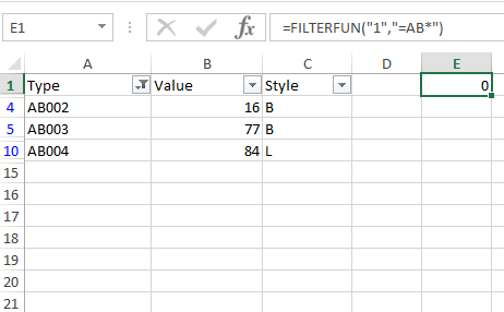
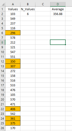
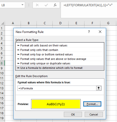
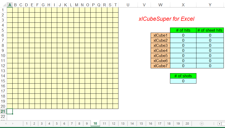
Due to some recent activity in the playing of this game, I started to think about any enhancements that would make the game easier to play. I realized that if a column was added to the scoring that showed the number of hits on each individual sheet for each cube, it would provide additional information to the player. So, my goal was to add that column, as shown in the figure below.

xlCube7_1

Initially, I thought that this would be a relatively simple task. However, I was wrong. The cube ships are laid out randomly as 3-D ranges. It is difficult or impossible to return the 2-D range associated with the 3-D range with normal worksheet formulas due to the limited ways to operate on 3-D ranges with worksheet functions. Thus, I realized that a UDF would be needed, since I did not want to modify the original programming. Then, I determined that the information that the UDF would require is:

  1. The 3-D range reference string.
  2. The “number” of the cube.
  3. The position(s) of the desired information in a 3-D range reference string.
  4. The first and last sheet of the 3-D range.
  5. The 2-D range associated with the 3-D range.
  6. The sheetname where it is being called from.

The complete code for the UDF is shown below.

Function SumSheetsHits()

Application.Volatile True

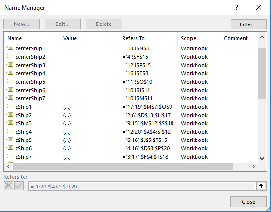
sRangeRaw = ThisWorkbook.Names(“cShip” & Application.Caller.Row – 5).RefersTo

sExclamation = Application.Find(“!”, sRangeRaw)

sColon = Application.Find(“:”, sRangeRaw)

sTick = InStr(sColon, sRangeRaw, “‘”)

If sColon = 4 Then

iFirst = Val(Mid(sRangeRaw, 3, 1))

Else

iFirst = Val(Mid(sRangeRaw, 3, 2))

End If

If sTick – sColon = 2 Then

iSecond = Val(Mid(sRangeRaw, sColon + 1, 1))

Else

iSecond = Val(Mid(sRangeRaw, sColon + 1, 2))

End If

aSheetNum = Val(ActiveSheet.Name)

srange = Mid(sRangeRaw, Application.Find(“!”, sRangeRaw) + 1, 255)

If aSheetNum < iFirst Or aSheetNum > iSecond Then

Else

SumSheetsHits = Application.Sum(ActiveSheet.Range(srange))

End If

End Function

So, the function =SumSheetsHits() is entered in column Y beginning on row 6. The line of code ThisWorkbook.Names(“cShip” & Application.Caller.Row – 5).RefersTo returns the 3-D formula string for cube 1 when entered in Y6. Application.Caller.Row is in row 6 in this example, so ThisWorkbook.Names(“cShip” & 6 – 5).RefersTo cShip1 and returns “ =’6:8’!$B$5:$D$7 “ which is the 3x3x3 cube 3-D reference.

Next, the 3 important characters for finding the desired information in the string are located. Note that both the FIND function and the InStr function are to find those positions, but really the InStr function could have been used for all 3 lookups.

sExclamation = Application.Find(“!”, sRangeRaw)

sColon = Application.Find(“:”, sRangeRaw)

sTick = InStr(sColon, sRangeRaw, “‘”)

The variable sTick shows the location of the 2nd tick in the string, since the search is made after the colon.

In order to find the first sheetname in the string (which by definition is a 1 or 2 digit number), this simple if, End if logic block of code is used.

If sColon = 4 Then

iFirst = Val(Mid(sRangeRaw, 3, 1))

Else

iFirst = Val(Mid(sRangeRaw, 3, 2))

End If

Note the use of the Val function, which converts the numeric string to an actual number. The find the second sheetname, the difference of sTick and sColon are used to define whether a 1 or 2 digit number is used.

If sTick – sColon = 2 Then

iSecond = Val(Mid(sRangeRaw, sColon + 1, 1))

Else

iSecond = Val(Mid(sRangeRaw, sColon + 1, 2))

End If

The sheetname is returned by the following code.

aSheetNum = Val(ActiveSheet.Name)

Since (fortuitously) the sheet names are consecutive numbers, that information makes the job of bounding the 3-D range much easier.

The 2-D range part of the formula is:

srange = Mid(sRangeRaw, Application.Find(“!”, sRangeRaw) + 1, 255)

and it is used with the final block of code.

If aSheetNum < iFirst Or aSheetNum > iSecond Then

Else

SumSheetsHits = Application.Sum(ActiveSheet.Range(srange))

End If


Since the 3-D range is bounded by these 2 sheets, any sheets outside would not be capable of recording any hits on this ship.

You might question the use of the SUM function here, when a hit on a ship appears as an “X”. Actually, when a shot is made, a 1 is placed in the cell, and the appearance of the “X” occurs through custom fomatting.

xlCubeSuper is now available with this new game functionaity, and can be downloaded by clicking the following link.

xlcubeSuper


Adding Data Validation to ANY Cell Using an Excel User-Defined Function


In previous articles I have written about the connection between Excel UDFs and objects, I have noted that almost any object can be invoked through its use. So, it was with interest that I read a recent article on Debra Dalgleish’s website on the accidental deletion of dropdown arrows when running macros.

https://contexturesblog.com/archives/2018/10/11/missing-data-validation-arrows/?utm_source=feedburner&utm_medium=feed&utm_campaign=Feed%3A+contextures%2FdCfy+%28Contextures+Blog%29

In the article, she stated

“If you run a macro that deletes shapes on a worksheet, it might also delete the drop down arrow. Excel sees that arrow as a worksheet shape.”

Well, I just wrote this article where a UDF invoked filter arrows to emulate the properties of Excel new FILTER function.

https://dhexcel1.wordpress.com/2018/09/30/the-new-microsoft-filter-and-sort-functions-are-great-but-what-about-the-old-ones-no-one-know-existed/

So, I figured that, just maybe, a UDF could do the same thing with data validation. It CAN! And, it can add the data validation to any desired worksheet cell.

The following code is for the AddValidation VBA UDF:

Function AddValidation(vRange As Range, vList As Range)

On Error Resume Next

Range(vRange.Address).Validation.Add Type:=xlValidateList, _

Formula1:=”=” & vList.Address

End Function

Its use can be seen in the following figures. In the first, the formula

=AddValidation(A3,letters) is in cell F5. Actually, in the figure the 2nd argument in the UDF is J1:J3, but that is equivalent to the defined name range called letters.

AddVal1

The first argument points to cell A3 as the target for adding the data validation list. In the 2nd figure, you can see that the data validation drowdown arrow appears in A3. Pretty amazing!

AddVal2

I think you can see the myriad of possibilties that are possible by using this technique.

Free free to download the sample workbook at the link shown below. HTH!

ValidationUDF

Excel Filter and Sort UDFs – Amazing!


In late September 2018, Microsoft revealed a number of fascinating new Excel worksheet functions.

https://techcommunity.microsoft.com/t5/Excel-Blog/Preview-of-Dynamic-Arrays-in-Excel/ba-p/252944

Bill Jelen has churned out an amazing 66-page ebook on the new functions.

https://www.mrexcel.com/download-center/books/2018/ExcelDynamicArraysStraightToThePoint.pdf

I strongly recommend that you look at the links listed above. Only then will you be able to appreciate what is presented in this article.

But, I don’t have immediate access to looking at these functions in the newest versions of Excel. So, that started me thinking: Could something similar to this work in a user-defined function (UDF)? My latest UDF creation, along with links to other interesting uses of UDFs can be viewed here.

https://dhexcel1.wordpress.com/2018/05/26/excel-generate-a-list-of-antonyms-using-an-user-defined-function-udf/

Well, to make a long story short, it can and furthermore they operate on the ORIGINAL DATA. This means they can filter a dataset in place and sort data in place instead of creating a duplicate dataset or subset like the new Excel functions do. You may ask how a UDF, entered in a worksheet cell remote for the data, can filter and/sort that table of data, and even I did not think that it was possible, or I would have exploited this long ago.

So, the FILTERFUN function presented here (I would have called it FILTER but I would not want it to conflict with the new Excel functions if used alongside them) can filter a table of data. In the figure shown below, the FILTERFUN function is shown along with a set of data. This UDF has 2 arguments, the field in the table to be filtered and the criteria to be used for the filter.

 AAA_ff01

If you are familiar with using Excel’s advanced data filter, you will note that the criterial in the 2nd argument uses the same syntax and has wildcard filtering abilities. The result for entering this formula can be seen in the next figure.

 AAA_ff02

The code for the FILTERFUN function fixes the location for the table to start in cell A1, but that can easily be modified, as can be seen in the code for the next magical UDF, the SORTFUN function.

This UDF has 3 arguments: the table range, the field to be used as the sort key, and the desired sort order, as shown:

 AAA_ff03

In this case, when the SORTFUN function is entered, the desired sort of the table is performed.

AAA_ff04

The following code for both of these functions is shown below.

 AAA_ff05

These functions provide a utility that can be made to mostly emulate the new Excel FILTER and SORT functions, while also allowing the desired result without creating new data tables.


I hope you find this technique useful. If so, share it with your Excel friends and colleagues.

The Excel file can be downloaded here:

FFunction


#Excel: Generate a List of Antonyms Using an User-Defined Function (UDF)

It really is amazing what you can do with an Excel user-defined function (UDF). Here is a list (not comprehensive) of articles from my website that demonstrate clever and unusual uses of UDFs.

https://dhexcel1.wordpress.com/2017/07/12/excel-short-and-sweet-tip-26-showing-an-userform-with-a-worksheet-udf-by-david-hager/

https://dhexcel1.wordpress.com/2017/07/07/excel-short-and-sweet-tip-25-playing-a-random-sound-with-a-worksheet-udf-by-david-hager/

https://dhexcel1.wordpress.com/2017/07/01/automating-word-and-powerpoint-from-excel-with-a-worksheet-udf-by-david-hager/

https://dhexcel1.wordpress.com/2017/06/19/excel-short-and-sweet-tip-23-open-windows-file-explorer-with-worksheet-udf-by-david-hager/

https://dhexcel1.wordpress.com/2017/06/07/excel-exchange-rate-udf-with-symbol-lookup-by-david-hager/

https://dhexcel1.wordpress.com/2017/06/03/creating-an-excel-translator-by-david-hager/

https://dhexcel1.wordpress.com/2017/05/23/excel-udf-using-google-api-to-return-the-elevation-of-an-address-by-david-hager/

https://dhexcel1.wordpress.com/2017/05/12/excel-creating-a-udf-with-the-vba-environ-function-and-using-it-to-make-a-table-of-environmental-variables-by-david-hager/

https://dhexcel1.wordpress.com/2017/04/29/excel-worksheet-udf-that-adds-a-comment-to-any-cell-by-david-hager/

https://dhexcel1.wordpress.com/2017/04/19/excel-modifying-shapes-from-an-udf-in-a-worksheet-cell-by-david-hager/

In this article, I will show how to use an Excel UDF to return a delimited string of antonyms. It uses Word VBA, so in order for the code to work, you must add a reference to the Microsoft Word Object library in the VBE, as shown below.

Antonym_VBE

Then, the following code for the UDF can be placed in a general module in the VBE.

Function AllAntonyms(TheWord As String)

Dim Alist

Alist = SynonymInfo(Word:=TheWord, LanguageID:=wdEnglishUS).AntonymList

For i = 1 To UBound(Alist)

If i = UBound(Alist) Then

DList = DList & Alist(i)

Else

DList = DList & Alist(i) & “,”

End If

Next

AllAntonyms = DList

End Function

The result for using this UDF in a worksheet cell with the word “excited” as the lookup for antonyms in shown in the following figure.

Antonym1

There are a number of possibilties for extending/modifying this example to other useful UDFs. I hope that you find this useful in that regard.

You can download the workbook here.


Thesaurus


xlCubeSuper An Excel Game Explained – Part6

This article is Part6 of a detailed explanation of the parts that went into the making of my xlCube game.

Sub NewGame()

Over = False

IniVar

ClearBoard

DeleteOldCubes

AskForGameLevel

tdAddNamedRanges

MakeCubeMenu

End Sub

The routine AskForGameLevel was needed in the older version of this game, but adding 2 more cubes changed my mind about having this option, so it is now set to 7 in this version.

The routine tdAddNamedRanges was discussed in a previous post in this series.


Sub IniVar()

hint1Val = 0

hint2Val = 0

hint3Val = 0

hint4Val = 0

hint5Val = 0

hint6Val = 0

hint7Val = 0

End Sub

This procedure simply sets variables used in the hint portion of the menu.

Sub ClearBoard() ‘prepares the worksheets for another game (some code can be cleaned up here)


Application.ScreenUpdating = False


For Each wsh In Sheets

wsh.Unprotect

Next


Sheets(Array(“1”, “2”, “3”, “4”, “5”, “6”, “7”, “8”, “9”, “10”, “11”, “12”, “13”, “14”, “15”, _

“16”, “17”, “18”, “19”, “20”)).Select


Sheets(“1”).Activate


With Range(“board”)

.ClearContents

.Font.ColorIndex = 1

ActiveWindow.SelectedSheets.FillAcrossSheets Range:=Range(“board”), Type:=xlAll

End With

This changes the font color for all cells in the board back to black.


Range(“A21”).Select

Sheets(“10”).Select


For Each wsh In Sheets

If wsh.Name <> “Scores” Then

wsh.Protect

End If

Next


Application.ScreenUpdating = True


End Sub


Sub DeleteOldCubes()

On Error Resume Next

With ThisWorkbook

For d = 1 To 7

.Names(“cShip” & d).Delete

.Names(“centerShip” & d).Delete

Next

End With

End Sub

Since the center of each cube is a named range, they can easily be deleted by using the Names property.


Sub MakeCubeMenu() ‘creates menu for xlCube

Dim xlCubeMenu As CommandBarPopup

DeleteCubeMenu ‘ deletes menu if it exists

Set xlCubeMenu = CommandBars(1).Controls.Add(Type:=msoControlPopup, temporary:=True)

xlCubeMenu.Caption = “&xlCube”

Set nGameMenuItem = xlCubeMenu.Controls.Add(Type:=msoControlButton)

With nGameMenuItem

.Caption = “&New Game”

.OnAction = “NewGame”

End With

For h = 1 To 7

Set nHintMenuItem = xlCubeMenu.Controls.Add(Type:=msoControlButton)

With nHintMenuItem

If h = 1 Then

.BeginGroup = True

End If

.Caption = “Hint: xlCube &” & h

.Tag = “Hint” & h

.OnAction = HINT_MACRONAME

.Parameter = h

EDMenuItem h ‘procedure that disables specified menu item if the corresponding cube has been destroyed

End With

Next

Set scoresMenuItem = xlCubeMenu.Controls.Add(Type:=msoControlButton)

With scoresMenuItem

.BeginGroup = True

.Caption = “&Scores”

.OnAction = “TheScores”

.Parameter = “Scores”

End With

Set instructMenuItem = xlCubeMenu.Controls.Add(Type:=msoControlButton)

With instructMenuItem

.BeginGroup = True

.Caption = “&Instructions”

.OnAction = “TheScores”

.Parameter = “Instructions”

End With

Set aboutMenuItem = xlCubeMenu.Controls.Add(Type:=msoControlButton)

With aboutMenuItem

.BeginGroup = True

.Caption = “&About xlCube”

.OnAction = “AboutThisGame”

End With

End Sub

This procedure adds the custom menu. Since this is an “old-style” menu, it appears on the Add-ins section of the ribbon.


I hoped you have enjoyed this series of articles on how I built this game.

xlCubeSuper An Excel Game Explained – Part5

The main explanation text for this article is in black and bold font. This is the primary procedure used in xlCubeSuper. When a cell is clicked, something happens depending on where it is and what it contains. The original documentation for this procedure is highlighted in green and other procedures used are highlighted in blue. They will be discussed in Part6.


“Shooting” is accomplished by this event procedure.


Private Sub Workbook_SheetSelectionChange(ByVal Sh As Object, ByVal Target As Excel.Range)


If Over Then Exit Sub ‘the Over variable is set to True when a game is finished


If ActiveSheet.Name = “Scores” Then Exit Sub ‘just in case you want to unhide this sheet

If Target.Font.ColorIndex > 1 Then Exit Sub ‘it already contains an “X”

If ActiveCell.Address <> Target.Address Then Exit Sub ‘if it is not a single cell selection

If Intersect(Range(“board”), Target) Is Nothing Then Exit Sub ‘if the selection is not on the board


Each of the 5 previous If-Then statement handle situations where the shot is not “correct”.


Calculate

NumOfHits = Application.WorksheetFunction.Sum(Range(“sumofhits”).Value) ‘hits before entry

On Error GoTo TheEnd

ActiveSheet.Unprotect


Target.Value = 1 ‘entry is made

This is prehaps the most important part of this procedure, although it looks very simple. It is, but adding a 1 to the cell does several things. First, it allows the formulas described in Part4 to keep track of all of the shots and hits. So, how does an X appear on the game board? Each cell has a custom format of “X”,,, which shows an X in the cell no matter what is entered.


Calculate

fShtPos = 0

TheRange = “”


The following loop checks to see whether the active cell is where any of the 7 centers of the cubes is located. If so, it will disable the hint in the menu associated with that cube and place a blue at that spot. Next, if the game is over (z=7) any hint costs will be summed and then added to the curent # of shots.


For p = 1 To 7


On Error Resume Next


tdRangeParse “centerShip” & p


If ActiveSheet.Name & Target.Address = fShtPos & TheRange Then ‘if a center of a cube has been hit


Target.Font.ColorIndex = 32

MsgBox “You just destroyed xlCube” & p & “!”, , “DESTROYED!”

Names(“cShip” & p).RefersTo = Range(“sums” & p).Value ‘changes name from reference to a value (# of hits)

Names(“centerShip” & p).Delete

Set cBar = Application.CommandBars.FindControl(Tag:=”Hint” & p)

cBar.Enabled = False ‘disables hint since corresponding cube is gone


For z = 1 To 7


If Mid(Names(“cShip” & z).RefersTo, 2, 1) = “‘” Then Exit For


If z = 7 Then

pScore = hint1Val + hint2Val + hint3Val + hint4Val + hint5Val + hint6Val + hint7Val ‘sums penalty score for hints

sScore = Range(“x15”).Value

fScore = pScore + sScore

MsgBox “The game is over! Your score is ” & fScore & “. ” & Chr(10) & Chr(13) & Level(fScore), , “GAME OVER!”

EnterInfo fScore

SortTable

ThisWorkbook.Save ‘saves changes made to records table

NewGame

Exit Sub

End If


Next


‘ActiveSheet.Protect

Exit Sub

End If


Next

If NumOfHits < Application.WorksheetFunction.Sum(Range(“sumofhits”).Value) Then

Target.Font.ColorIndex = 3 ‘turns red if hits > before event

End If


Finally, if the the shot is a hit, it will change the font color to red.


ActiveSheet.Protect

TheEnd:

End Sub


Although I have not explained every aspect of this procedure, I hope that this helps!

xlCubeSuper An Excel Game Explained – Part4

This is the 4th post to explain in detail how my xlCube game application was constructed. To read the previous post, go to:

https://dhexcel1.wordpress.com/2018/01/21/xlcubesuper-an-excel-game-explained-part3/

The number of hits is recorded by this formula

=SUM(BigBoard)

Where BigBoard is the 3D range representing the playing board.

The number of shots is recorded by this type of formula for each of the 7 cubes.

=IF(ISNA(ERROR.TYPE(cShip7)),SUM(cShip7),IF(ERROR.TYPE(cShip7)=5,0,SUM(cShip7)))

For explanation of the ERROR.TYPE function, see:

https://support.office.com/en-us/article/ERROR-TYPE-function-10958677-7c8d-44f7-ae77-b9a9ee6eefaa?NS=EXCEL&Version=16&SysLcid=1033&UiLcid=1033&AppVer=ZXL160&HelpId=xlmain11.chm60309&ui=en-US&rs=en-US&ad=US

See the figure for each area discussed.

 xlCS4_Board

The following formulas use the EVALUATE function, which is an old-style xlm macro function. It can only be used in a defined name formula. If you have noticed an issue opening the game application, this may be the cause. You would then have to place the file in a trusted location to open it. They are used in the conditional formatting of the 7 hits cells.

gbool1 =ERROR.TYPE(EVALUATE(“cShip”&ROW()-5))=5

This formula is really just there in case there is no ship center for that specific ship. Previously, the user was allowed to select the number of ships to be created, so this conditional formatting formula is really a legacy feature, not affecting the game functionality.

gbool2 =NOT(ISERROR(EVALUATE(“cShip”&ROW()-5)))

If the cell for cShip1 (in row 6) has a black color from conditional formatting, it means that this formula is TRUE, cShip1 does not exist. It has been destroyed.

The next post will focus on “taking a shot”.


xlCubeSuper An Excel Game Explained – Part3

This is the 3rd post to explain in detail how my xlCube game application was constructed. To read the previous post, go to:

https://dhexcel1.wordpress.com/2018/01/20/xlcubesuper-an-excel-game-explained-part2/

This is the VBA routine I developed to add 3D cube ranges to the playing board of xlCubeSuper. It generates 7 3D ranges randomly with sizes ranging from 3x3x3 to 15x15x15.

Sub tdAddNamedRanges()

Randomize ‘ Initialize random-number generator

For s = 1 To 7

‘set x,y, and z values to fall within limits determined by cube size

x = 1 + Int(Rnd() * (20 – (2 * s)))

y = 1 + Int(Rnd() * (20 – (2 * s)))

z = 1 + Int(Rnd() * (20 – (2 * s)))

‘create R1C1 style formula strings

cShipStr = “='” & z & “:” & z + (2 * s) & “‘!R” & x & “C” & y & “:R” & x + (2 * s) & “C” & y + (2 * s)

centerShipStr = “='” & z + s & “‘!R” & x + s & “C” & y + s

‘create names for cube 3D references and the centers of each cube

matchVar = False

With ThisWorkbook.Names

.Add Name:=”cShip” & s, RefersToR1C1:=cShipStr, Visible:=False

.Add Name:=”centerShip” & s, RefersToR1C1:=centerShipStr, Visible:=False

End With

If s > 1 Then

For m = 1 To s – 1

If Names(“centership” & m).RefersTo = Names(“centership” & s).RefersTo Then

matchVar = True

End If

Next

End If

If matchVar Then

s = s – 1

End If

Next

End Sub

The first statement in the VBA procedure uses RANDOMIZE to create a numeric seed that will be used by the RND function to generate a random number.

Inside the For-Next statement, which sets the variable “s” to a value from 1 to 7, the xyz coordinates for each cube are generated as follows:

x = 1 + Int(Rnd() * (20 – (2 * s)))

y = 1 + Int(Rnd() * (20 – (2 * s)))

z = 1 + Int(Rnd() * (20 – (2 * s)))

The numbers generated by these fomulas keep the cube on the board, depending on the value of “s”. The z coordinate is for the worksheets included in tne board and the xy coordinates are for the cells.

Then, for each value of “s”, the 3D cubical range and the center of each cube are generated with these formulas in R1C1 format.

cShipStr = “='” & z & “:” & z + (2 * s) & “‘!R” & x & “C” & y & “:R” & x + (2 * s) & “C” & y + (2 * s)

centerShipStr = “='” & z + s & “‘!R” & x + s & “C” & y + s

When they are saved as defined name formulas using the following code,

With ThisWorkbook.Names

.Add Name:=”cShip” & s, RefersToR1C1:=cShipStr, Visible:=False

.Add Name:=”centerShip” & s, RefersToR1C1:=centerShipStr, Visible:=False

End With

the formulas are converted by Excel into A1 format.

Originally, this was all of the code for this process. What I had ignored what the fact that two different cubes could have the exact same center. During all of the testing/playing of this game over the years, that scenario was never recognized as having occurred. But the current version, with 7 cubes, had this happen several times in early testing. So, I came up with this solution to correct this issue.

If s > 1 Then

For m = 1 To s – 1

If Names(“centership” & m).RefersTo = Names(“centership” & s).RefersTo Then

matchVar = True

End If

Next

End If

If matchVar Then

s = s – 1

End If

A key part to this code is

Names(“centership” & m).RefersTo = Names(“centership” & s).RefersTo

which compares the currently added formula to each previous formula added. If this statement is TRUE, then matchVar is set to TRUE. Then,

If matchVar Then

s = s – 1

End If

which decrements “s” by 1, effectively rerunning the previously generated 3D formula until an unique center is produced.

The next post will discuss the worksheet formulas used in this game.


xlCubeSuper An Excel Game Explained – Part2

In Part1, the new version of xlCube (now referred to as xlCubeSuper) was introduced.

https://dhexcel1.wordpress.com/2018/01/19/xlcubesuper-an-excel-game-explained-part1/

In Part2, I will describe the different techniques to make this game application work. But, before I do, I think that it is important to point out that the game is not tied down tight. For example, there is no workbook-level protection. If users wanted to, they could damage the integrity of the game by adding or deleting worksheets (if they saved the changes). So, the game is not tamper-proof and was never intended to be. Rather, it was made as a game to be enjoyed and an application to learn from. Here then is a list of the major techniques to be discussed.

  • 3D formulas
  • Defined named formulas
  • Conditional formatting formulas
  • Formulas to aggregate shots and hits
  • Use of VBA to:
  1. Add 3D ranges
  2. Shoot using VBA event procedure.
  3. Create and delete non-ribbon (old style) menus.
  4. Store and sort game scores.
  5. Control the formatting of shots and hits.
  6. Display information and results.

The backbone of this game is the 3D formulas created to define virtual cubes and the center of those cubes. We will see in a later post how these formulas are generated through VBA, but for now, here is what they look like as shown in Name Manager.

xlCS2_3Dformulas

In Part3 we will see how these formulas are created in random locations by VBA.

xlCubeSuper An Excel Game Explained – Part1

I have just recently updated/modified my xlCube game that I first started on 20 years ago. The main modification is that it now has 7 cubes that must be destroyed before the game is over. For those who have never played the game, the previous version can be found at:

https://dhexcel1.wordpress.com/2016/11/29/xlcube-an-excel-game/

The new game is called xlCubeSuper. And, like the previous release, I encourage you to dig into the details of how this application was constructed. But, I know that your time is precious, and you may feel that this would not be an effective use of your Excel time. So, this time I am going to explain in detail all of the tricks and techniques used in the making of this game. In Part 1, I am only making it available to you. The explanation will come in subsequent posts. In the meantime, have fun with it.

You can download the file here.

xlcubeSuper


#Excel Data Validation – Non-Contiguous Ranges and Changing Data Validation List after Picking

I recently saw this challenge for creating a data validation list from 2 non-contiguous ranges.

https://www.sumproduct.com/blog/article/monday-morning-mulling-december-challenge

Then, while looking up current information about data validation tricks, I reread this post on Debra Dalgleish’s Excel site, which showes a way to change the data validation list based on items picked.

http://www.contextures.com/xlDataVal03.html

I decided that I would try to combine both of these techniques, while at the same time creating the required data validation list without the need for helper columns. When I started on this, I was not sure that it would be possible, but that is the kind of challenge I like 😊.

I had previously published a method for combining non-contiguous ranges into a comma-delimited string.

https://dhexcel1.wordpress.com/2017/05/21/excel-short-and-sweet-tip-15-using-textjoin-with-non-contiguous-ranges-by-david-hager/

Using this technique along with modifying the ranges to exclude blank values, the following formula produces a delimited string combining the elements of two ranges named List1 and List2, as shown in the figure.

DV_PIC1

TJ_TLists =TEXTJOIN(“,”,TRUE,IF(ISBLANK(List1),””,List1),IF(ISBLANK(List2),””,List2))

It is important to note here that any number of ranges (rectangular, non-contiguous or 3D) can be combined in this step to afford the data validation list in the final step. As an example, see:

https://dhexcel1.wordpress.com/2017/05/23/excel-native-3d-ranges-with-the-textjoin-function-plus-bonus-by-david-hager/

The next formula converts this delimited string into an array.

CombinedDV =TRIM(MID(SUBSTITUTE(TJ_TLists,”,”,REPT(” “,999)),ROW(INDIRECT(“1:”&LEN(TJ_TLists)-LEN(SUBSTITUTE(TJ_TLists,”,”,””))+1))*999-998,999))

Unfortunately, an array cannot be used directly as a data validation list. But, since there is more work to do to create data validation that can be used as a pick list, the following formulas are needed.

MatchArr=IF(ISNA(MATCH(ROW(INDIRECT(“1:”&COUNTA(CombinedDV))),MATCH(SelectDV,CombinedDV,0),0)),CombinedDV,””)

affords {“”;”b”;”c”;”d”;”e”;”f”;”g”;”h”;”I”;”j”;”k”;”l”;”m”;”n”;””}

MatchRow=IF(ISNA(MATCH(ROW(INDIRECT(“1:”&COUNTA(CombinedDV))),MATCH(SelectDV,CombinedDV,0),0)),ROW(INDIRECT(“1:”&COUNTA(CombinedDV))),””)

affords {“”;2;3;4;5;6;7;8;9;10;11;12;13;14;””}

Then in cell H2 is entered the formula =INDEX(MatchArr,SMALL(MatchRow,ROW()-1)),which is filled down until a formula returns an error. This is the range to be used as a data validation list.

As shown in the figure, the range where data validation is applied

SelectDV=DVSheet!$B$2:$B$16

contains an “a” and an “o”.

Then, the formula used for the data validation list is

DVList=DVSheet!$H$2:INDEX(DVSheet!$H$1:$H$16,MATCH(TRUE,ISERROR(DVSheet!$H$1:$H$16),0)-1)

So, when the data validation is used in its current state, the list will not contain those two letters.

I hope that you find this useful.

The example file can be downloaded here.

DV_TwoLists

#Excel: Extracting an Array of Words From a Sentence


The following formula will create an array of words from a string (sentence).

= ArrayFromSDS(TEXTJOIN(“”,,IF(MID(A1,ROW(INDIRECT(“1:”&LEN(A1))),1)=” “,” “,IFERROR(CHAR(64+MATCH(MID(SUBSTITUTE(SUBSTITUTE(A1,”?”,”-“),”*”,”-“),ROW(INDIRECT(“1:”&LEN(A1))),1),CHAR(64+ROW(INDIRECT(“$1:$26″))),0)),””))))

Here is an explanation of how it works.

The array used in the 3rd argument of the TEXTJOIN function starts with the 1st part of the IF formula, shown below.

IF(MID(A1,ROW(INDIRECT(“1:”&LEN(A1))),1)=” “,” “,

which keeps any space from the string in cell A1. The rest of the IF formula

IFERROR(CHAR(64+MATCH(MID(SUBSTITUTE(SUBSTITUTE(A1,”?”,”-“),”*”,”-“),ROW(INDIRECT(“1:”&LEN(A1))),1),CHAR(64+ROW(INDIRECT(“$1:$26″))),0)),””)

returns only letters from the string in A1. The 1st argument of the MATCH function in this construction,

MID(SUBSTITUTE(SUBSTITUTE(A1,”?”,”-“),”*”,”-“), ROW(INDIRECT(“1:”&LEN(A1))),1)

is very similar to the 1st part of the IF function, but it has one important difference.

Instead of using the string from cell A1, the formula SUBSTITUTE(SUBSTITUTE(A1,”?”,”-“),”*”,”-“) is used instead. The reason for doing this is that the MATCH function recognizes the * and ? symbols as wildcard searches. So, if the 2nd argument of the MATCH function does NOT contain a * or ?, the character “A” will be returned instead (if not removed from the core string).

The 2nd argument of the MATCH function is

CHAR(64+ROW(INDIRECT(“$1:$26”)))

which returns an array of letters from A TO Z.

The result of the MATCH function is an array with numbers from 1-26 for positions in the string with letters and “” if not. For example, if the string in A1 is “ AAx,d a.”x~y*z”. c?e! ”, then the MATCH array will return

{1;1;24;#N/A;4;#N/A;1;#N/A;#N/A;24;#N/A;25;#N/A;26;#N/A;#N/A;#N/A;3;#N/A;5;#N/A}

This array is particularly useful in this specific case, since the numbers can be converted to the letters in the string by using the CHAR function (along with the IFERROR function to turn errors to an empty string). That converts the array to

{“A”;”A”;”X”;””;”D”;” “;”A”;””;””;”X”;””;”Y”;””;”Z”;””;””;” “;”C”;””;”E”;””}

Now, this array can be used as the main argument in the TEXTJOIN function to afford the string

AAXD AXYZ CE

Now, using the ArrayFromSDS user-defined function (shown below)

Function ArrayFromSDS(MyString As String)

ArrayFromSDS = Split(MyString, ” “)

End Function

produces this array of words.

{“AAXD”,”AXYZ”,”CE”}

HTH!


#Excel: Remove Multiple Characters From a String Using The TEXTJOIN Function and Without Using the SUBSTITUTE or REPLACE Function


There are a number of examples of the removal of characters from a string which utilize nested SUBSTITUTE or REPLACE functions. However, they are hard-coded in that the formulas are built with a set number of characters to remove based on the times that the SUBSTITUTE function is used. The formula methodology I am presenting here is more flexible and robust than previous solutions.

In this example, I am trying to remove all punctuation from a string, specifically the one shown below from cell A1. You will note that this string contains five different punctuation symbols, several occurring more than once.

x,da.”xyz”.c?e!

The following array formula removes those symbols

=TEXTJOIN(“”,TRUE,IF(ISERROR(MATCH(MID(A1,ROW(INDIRECT(“1:”&LEN(A1))),1),{“,”;”.”;”?”;”!”;””””},0)),MID(A1,ROW(INDIRECT(“1:”&LEN(A1))),1),””))

and affords the desired string shown below.

xdaxyzce

HTH!

#Excel: Most Frequent Item in a List of Delimited Strings


rng is a defined name range on the worksheet with each cell containing delimited strings. Although it does not necessarily have to be a 1-column list, most examples of delimited strings in a range are of this type. To convert this range to an array, use the following formula.

Define arr as =ArrayFromCDS(TEXTJOIN(“,”,,rng))

where the VBA UDF is shown below.

Function ArrayFromCDS(MyString As String)

ArrayFromCDS = Split(MyString, “,”)

End Function

So, arr is a 1-D array of all of the delimited values from each cell of the range. Then, use this formula

=INDEX(arr,MODE(MATCH(arr,arr,0)))

to return the most frequent item.

Insert a Line-Feed Between Every 3rd Character Using an Excel Worksheet Formula


Per an Oz Du Soleil post on how to separate 5 area codes in a single 15 character string with line breaks using Power Query

https://m.youtube.com/watch?v=yorGlCrfqY0  

here is a way to do the same thing using a worksheet formula.

With the string in cell A1. Enter the following array formula in a cell.

=TEXTJOIN(CHAR(10),,MID(A1,{1,4,7,10,13},3))

Make sure that you select word wrap enabled for the cell containing the formula.

Boolean Formula for Repetitive Characters in a String

  • My answer to a Chandoo challenge. Not exactly the question most are answering, however. More robust. So, the string “hellp” (in cell A1) would return TRUE but “helpl” would return FALSE. I chose the degree symbol (Alt 0176) as my unlikely used twice in a row character, but you can choose another.

=NOT(ISERROR(MATCH(TRUE,CODE(MID(A1,ROW(OFFSET($A$1,,,LEN($A$1))),1))*2=CODE(MID(A1&”°”,ROW(OFFSET($A$1,,,LEN($A$1))),1))+CODE(MID(A1&”°”,ROW(OFFSET($A$2,,,LEN($A$1))),1)),0)))  CSE

#Excel Short and Sweet Tip #29: Inserting Icons Using a User-Defined Function

Disclaimer: You need the Excel version included in Office 365 for this technique to work.

The insertion of icons in Excel 2016 is accomplished from the ribbon by selecting Insert, Icons. There are a number of catagories to select from, as shown in ths figure.

MakeIcon1

However, recently I have been interested (obsessed?) with worksheet UDFs and their ability to invoke actions or shapes. In this case, I wanted to see if a UDF would insert an icon into the worksheet. This is the VBA function I made with help of the macro recorder. Place this in a general module in your worksheet.

Function MakeIcon(fName As String)

iString =        “https://hubblecontent.osi.office.net/ContentSVC/Content/Download?provider=MicrosoftIcon&amp;

fileName=” & fName & “.svg”

ActiveSheet.Pictures.Insert iString

End Function

Now, enter the formula =MakeIcon(“Man”) in cell A1 and you will get the following result.

MakeIcon

Unfortunately, there are several inherent Excel limitations that prevent the full utilization of this function. First, you have to know the correct name of the icon to produce it. It would be nice if Microsoft provided a list of the icon names, but I could not locate one. Then, I tried to get names by macro recording the insertion of multiple icons, but only the “last” selected icon URL is recorded. Even so, I hope that this technique is useful to you.

The example file can be downloaded here.

MakeIcon

Generating a “Realtime” Voice Alert for the Latest Magnitude 5 or Greater Earthquake


I recently published an article about getting information on the latest earthquake of magnitude 5 or greater.

https://dhexcel1.wordpress.com/2017/07/10/getting-the-latest-earthquake-alert-using-the-webservice-and-filterxml-functions-in-excel-by-david-hager/

Please read this article to see how the core model was constructed.

One problem with this model is that since Excel’s web functions are non-volatile, a formula containing those functions must be recalculated by reentering the formula. I decided that an easier way was needed to trigger an update. I also recently published an article which utilized the hyperlink rollover technique.

https://dhexcel1.wordpress.com/2017/09/15/highlighting-words-in-an-excel-list-using-the-hyperlink-rollover-method/

I figured that this might be a good way to trigger a recalculation. And, since I was going to use a VBA function to be called from the hyperlink formula, I thought that adding audio functionality would be useful as well. Here is the hyperlink rollover formula used (in cell D5, named Recalculate). Since a rollover is required, the technique is not truly realtime.

=IFERROR(HYPERLINK(EarthQuakeAlert(),”Recalculate”),”Recalculate”)

And, here is the VBA function called by “rolling over” (passing the cursor over) that cell.

Function EarthQuakeAlert(Optional Person As String = “Him”, _

Optional Rate As Long = 1, Optional Volume As Long = 80)

Static xlApp As New Excel.Application

Dim Voc As SpeechLib.SpVoice

Set Voc = New SpVoice

Dim sAddress As String

‘Application.Volatile True

xlApp.CalculateFull

If Range(“d1”).Value = Range(“b3”).Value Then

MsgBox “No new earthquake > 5.0”

Else

With Voc

If Person = “Him” Then

Set .voice = .GetVoices.Item(0) ‘male

ElseIf Person = “Her” Then

Set .voice = .GetVoices.Item(1) ‘female

Else

End If

.Rate = Rate

.Volume = Volume

.Speak “New Earthquake Alert! ” & Range(“b5”).Value

End With

Range(“d1”).Value = Range(“b3”).Value

End If

EarthQuakeAlert = “Recalculate”

Set xlApp = Nothing

End Function

In order to use SpeechLib.SpVoice in the code, the correct reference (from Tools, References) must be added to the VBE as shown in the following figure.

AudioEarthquakeAlert1

In this figure is a picture of the earthquake model.

AudioEarthquakeAlert2

I hope that you find this useful. You can download the file here.

earthquake_audio­_alert

Get Latest Storm Information in #Excel Using Only An Address and Storm Name


I recently published this article about the direction and distance of a tropical system from an address.

https://dhexcel1.wordpress.com/2017/09/12/using-excel-to-find-how-far-the-storm-is-from-your-location/

Go back and read this article to understand the first part of the model associated with the address (entered manually in cell B1).

Originally I wanted to include the abilty to add the storm coordinates from an internet source but I could not find one, so manually entering them was necessary. However, later I stumbled across just the xml source I was looking for from the National Hurricane Center site at NOAA. It only gives the current information on a storm, so it gets “stepped on” with each new advisory. This information is for storm number 15 for the 2017 Altantic hurricane season, which hhappens to be Maria.

http://www.nhc.noaa.gov/storm_graphics/AT15/atcf-al152017.xml

In order to access more than one system, I replaced the number with a defined name function called StormNum, which is then used as the URL in the WEBSERVICE function to return the desired xml document.

=WEBSERVICE(“http://www.nhc.noaa.gov/storm_graphics/AT”&StormNum&”/atcf-al”&StormNum&”2017.xml”)

I also needed a list of the storms for 2017. One complication was that the NHC now gives Potential Tropical Cyclones a number like those given to all tropical lows. Then, if the PTC does not develop into a low pressure system, it will not show up in online lists, like for example, Wikipedia. However, I was able to find a site that did include PTCs and I used Power Query to get the table containing the desired information (see worksheet SysNames). I massaged the column containing the storm designations as shown in column G. The formula used for this is =IF(PROPER(TRIM(RIGHT(SUBSTITUTE(A3,” “,REPT(” “,100)),100)))=””,”Not Yet”,PROPER(TRIM(RIGHT(SUBSTITUTE(A3,” “,REPT(” “,100)),100)))). Shown below:

 StormUpdate2

The source from the PQ M code is:

=Web.Page(Web.Contents(“http://www.theweatherguys.com/index.php?config=&forecast=tropsystems&alt=tropallsystems&#8221;))

Now that I had the list of storms, I was able to construct the StormNum defined name formula as follows:

=IF(Storm_Number<10,”0″&Storm_Number,Storm_Number)

where Storm_Number =MATCH(DirectionCalc!$B$2,Storm_List,0). Cell B2 contains a data validation list with the storm names derived from the PQ.

Now, the FILTERXML function can extract various pieces of information from the xml doucment defined as Storm, as shown in the following figure.

 StormUpdate1

For example, the storm latitude (in cell C4) is =FILTERXML(Storm,”//centerLocLatitude”).

The final formula for the storm message is:

=ROUND(Distance,0)&” miles “&TextDirection&” of “&Address&”, moving “&MID(FILTERXML(Storm,”//systemDirectionOfMotion”),1,FIND(“OR”,FILTERXML(Storm,”//systemDirectionOfMotion”))-1)&”at “&FILTERXML(Storm,”//systemSpeedMph”)&” mph.”

Remember, do no use this model in any corporate or commercial manner (only for personal use).

You can download the file here.

DirectionFromStorm_AutoLookup

Highlighting Actual Words in an #Excel List Using the Hyperlink Rollover Method

The Hyperlink Rollover technique was discovered by Jordan Goldmeier. It uses the HYPERLINK function with a VBA function procedure as the 1st argument. By passing the cursor over the cell containing this formula, the function procedure is run. See:

http://optionexplicitvba.blogspot.com/2011/04/rollover-b8-ov1.html

And, this function, unlike normal UDFs, can modify the Excel worksheet.

I have been trying for quite some time to develop a way to highlight (format) cells in a list that contain words. It turns out that there is a bug (feature?) in the VBA expression Application.CheckSpelling that prevents its use in an UDF. For example, if I wanted to conditionally format cell A1 to highlight a string that is a word, you might expect that the following UDF could be used as a CF formula.

Function IsWord(WordRange As Range)

IsWord = Application.CheckSpelling(WordRange)

End Function

Well, it does not work. The problem is documented at the following link.

https://stackoverflow.com/questions/10776191/spellcheck-a-single-word-in-excel-function

I tried numerous methods to find something that would work. I won’t bore you with the details, but I used a lot of time on this without success. I even used the Hyperlink Rollover method, and it still did not work. Finally, in the last comment in the link shown above, I found that an early binding process was needed. When added to the regular UDF for use in conditional formatting, it still did not work, but it did work with Hyperlink Rollover. Here is the UDF developed to highlight words:

Function IsWord(WordRange As Range)

Static xlApp As New Excel.Application

For Each cRange In WordRange

If xlApp.CheckSpelling(cRange) Then

With cRange.Font

.Color = -16776961

.Bold = True

End With

End If

Next

IsWord = 0

Set xlApp = Nothing

End Function

By using this UDF with this technique, the following formula entered In cell D1 creates the Hyperlink Rollover location.

=IFERROR(HYPERLINK(IsWord(A1:A20),”Format Words”),”Format Words”)

After passing the cursor over this cell, the result can be viewed in the following figure.

HyperLinkRolloverWord1

I decided to add another word to that range in cell A9. Without “rolling over”, this cell now showed that A9 contained a word.

HyperLinkRolloverWord2

I was rather amazed by this. I could not find an example of this in any previous Hyperlink Rollover, but I might have missed seeing it. What I believe is occurring is that any change in the range used in the IsWord function serves as the same action as a rollover. I did verify that this condition persists even after the workbook is closed and reopened.

So…

I decided to use a dynamic range as the argument in the IsWord function, as shown below.

=IFERROR(HYPERLINK(IsWord(OFFSET(A1,,,COUNTA(A:A),)),”Format Words”),”Format Words”)

By adding several more cells with strings, the figure below shows the results.

HyperLinkRolloverWord3

I hope that you find this technique useful.

You can download the example file here.

IsWord

Using #Excel to Find How Far the Event is from Your Location

Note: It is important to note that this Excel model can be used any place in the world to look at the direction from storms or any other event.

 The destructive nature of hurricanes has been dominating the news recently in the Atlantic basin. But, many times it is difficult to get information about how far a storm is from your specific location. This excellent Excel technique will allow you to answer that question. All that you will need is your address (or an address of interest) and the current storm coordinates. Key parts of this technique were found at the following links.

https://chandoo.org/forum/threads/using-excel-to-find-lat-and-long-from-a-street-address-geocode.9793/

https://www.mrexcel.com/forum/excel-questions/541185-convert-number-deg-direction-text-n-nne.html

In the worbook provided, enter your address information in cell B1and the storm coordinates in C4 and D4. The formulas used to calculate your result are:

LocationXML =WEBSERVICE(“http://maps.googleapis.com/maps/api/geocode/xml?address=”&Address&”+,+&sensor=false&#8221;)

Lat_1 =FILTERXML(LocationXML,”//result/geometry/location/lat”)

Lng_1=FILTERXML(LocationXML,”//result/geometry/location/lng”)

Distance=ACOS(SIN(Latitude_1*PI_DIV180)*SIN(Latitude_2*PI_DIV180)+COS(Latitude_1*PI_DIV180)*COS(Latitude_2*PI_DIV180)*COS((Longitude_2*PI_DIV180)-(Longitude_1*PI_DIV180)))*3959

PI_DIV180=PI()/180

Direction =DEGREES(ATAN2(COS(RADIANS(Latitude_1))*SIN(RADIANS(Latitude_2))-SIN(RADIANS(Latitude_1))*COS(RADIANS(Latitude_2))*COS(RADIANS(Longitude_2-Longitude_1)),SIN(RADIANS(Longitude_2-Longitude_1))*COS(RADIANS(Latitude_2))))

TextDirection=CHOOSE(1+ROUND(IF(Direction<0,360+Direction,Direction)/22.5,0),”N”,”NNE”,”NE”,”ENE”,”E”,”ESE”,”SE”,”SSE”,”S”,”SSW”,”SW”,”WSW”,”W”,”WNW”,”NW”,”NNW”,”N”)

The final formula for displaying the desired information (in cell A7) is:

=ROUND(Distance,0)&” miles “&TextDirection&” of “&Address

The result can be viewed here.

DirectionFromStorm1

I hope that you find this useful. Download the example file:

DirectionFromStorm


#Excel Advanced Filter: Selectively Show Control Chart Data by Standard Deviation


For this technique, I am building it on the workbook made for the following article. Please download the example file and read the article, since the functionality is synergistic with it.

https://dhexcel1.wordpress.com/2017/05/17/excel-modifying-control-chart-data-to-remove-outliers-with-excel-formulas-by-david-hager/

When viewing a control chart, it is useful to be able to view only data within set control limits. For example, you would like to view all data within one sigma of the mean. The technique described here allows you to do that for 1, 2, or 3 sigma. The key to accomplish this is Excel’s advanced data filter. The advanced filter uses a boolean formula to filter a table of data, starting at the first row of the table. The formula in A2 gives the desired result.

=AND(B6<CHOOSE(SigmaKeep,D6,E6,F6),B6>CHOOSE(SigmaKeep,G6,H6,I6))

where SigmaKeep is a worksheet cell (G2) with a data validation list of 1,2,3. Cells D6 and G6 (and the corresponding columns) contain formulas that calculate the +1 and -1 sigma from the mean for the data in column B. The 2nd and 3rd sigma are for E6,H6 and F6,I6 respectively. The following figure shows the advanced filter dialog box and the input ranges required, where SigmaKeep is set at a value of 2.

 ModifyStdData_AdvFilter1

After the filter is applied, note the difference in the data in the control chart versus the original in the first figure.

 ModifyStdData_AdvFilter2

The only caveat to this technique is that the advanced filter has to be cleared (Data, Sort & Filter, Clear) before a different KeepSigma value can be applied. This can be used in conjunction with the removal of outliers as discussed in the original article.

The example file can be downloaded here.

ModifyStdData_AdvFilter


Adding Multiple DAX Measures to Non-PowerPivot Versions of #Excel using an User-Defined VBA Function


In this article,

http://dailydoseofexcel.com/archives/2017/07/10/look-ma-no-powerpivot/

Jeff Weir pointed to a video made by Mike Girvin about adding measures to non-PowerPivot versions of Excel (link below)

https://www.youtube.com/watch?v=FVVK-8QZC1M&t=422s

Mike demonstrated how measures can be added to a data model in these “disabled” version through pivot table options. Please view this video to see how Mike did it.

The link to the working file for this video will be referred to in this article (Thanks, Mike!).

https://people.highline.edu/mgirvin/YouTubeExcelIsFun/EMT1269Finished.xlsx

You can download this file and reproduce the technique presented here.

Although it is not well-known, Microsoft started at Excel version 2016 (Office 365) marketing versions that do not have PowerPivot capability. For details on this, see:

https://blogs.office.com/en-us/2015/09/18/new-ways-to-get-the-excel-business-analytics-features-you-need/

So, this article is dedicated to those who purchased non-PowerPivot versions of Excel 2016, although the technique presented here will work on any version of Excel 2013 or greater.

Jeff Weir mentioned in his article that since some Excel 2016 versions did not have the full-blown PowerPivot capability, and that VBA could be used to build a user interface to the data model. Well, I have not created a UI, but I have made a way to add multiple measures to the data model using an user-defined function. The code for the VBA function is shown below. To use this, add astandard module in the VBE and then save the workbook as .xlsm. Then, copy/paste the code into the module.


Function AddMeasure(TableName As String, MeasureName As Range)

Application.Volatile False

With ActiveWorkbook.Model

For Each mCell In MeasureName

mFormat = mCell.Offset(0, 2).Value

.ModelMeasures.Add mCell.Value, .ModelTables(TableName), mCell.Offset(0, 1).Value, _

Switch(mFormat = “Boolean”, .ModelFormatBoolean, mFormat = “Currency”, .ModelFormatCurrency, _

mFormat = “Date”, .ModelFormatDate, mFormat = “DecimalNumber”, .ModelFormatDecimalNumber, _

mFormat = “General”, .ModelFormatGeneral, mFormat = “PercentageNumber”, .ModelFormatPercentageNumber, _

mFormat = “ScientificNumber”, .ModelFormatScientificNumber, mFormat = “WholeNumber”, .ModelFormatWholeNumber), _

mCell.Value

Next

End With

AddMeasure = “DONE”

End Function

Then, place the following information in the range D10:F14.


NetRevenue SUMX(fTransactions,ROUND(RELATED(dProducts[Price])*fTransactions[Units]*(1-fTransactions[Discount]),2)) DecimalNumber
MaxRevenue MAXX(fTransactions,ROUND(RELATED(dProducts[Price])*fTransactions[Units]*(1-fTransactions[Discount]),2)) PercentageNumber
MinRevenue MINX(fTransactions,ROUND(RELATED(dProducts[Price])*fTransactions[Units]*(1-fTransactions[Discount]),2)) Currency
AverageRevenue AVERAGEX(fTransactions,ROUND(RELATED(dProducts[Price])*fTransactions[Units]*(1-fTransactions[Discount]),2)) General
CountOfRevenue COUNTAX(fTransactions,ROUND(RELATED(dProducts[Price])*fTransactions[Units]*(1-fTransactions[Discount]),2)) General


To run this as a worksheet formula, type this formula in any cell.

=AddMeasure(“fTransactions”,D10:D14)

This will add the 5 measures to the data model, as shown in the Pivot Table Fields list.

AddMeasure2

After the 5 measures are added to the pivot table, the resulting pivot table will look like this.

AddMeasure5

Of course, the DAX formulas to be added have to return valid results, or the procedure will fail.

This powerful technique is yet another reason why users should not completely abandon Excel for Power BI desktop, as discussed in this article at powerpivotpro.com

https://powerpivotpro.com/2017/09/excel-is-still-the-best-tool-for-teaching-dax/

And, this technique does not HAVE to be run from a UDF, but I am still amazed that it can. I am sure that you will find this very useful.

#Excel Impossibly Easy #2: Change Sheet Tab Color with a User-Defined Worksheet Formula

What if I told you that I wanted to change tab colors on sheets in a workbook by entering a formula (UDF) on a worksheet. Impossible, right? No, it turns out that it is “easy”.

This simple UDF (code shown below) can be entered on a worksheet and the desired worksheet tab will change to any color you want.

Function ChangeTabColor(sht As String, RED_Color As Integer, GREEN_Color As Integer, BLUE_Color As Integer)

With ActiveWorkbook.Sheets(sht).Tab

.Color = RGB(RED_Color, GREEN_Color, BLUE_Color)

End With

End Function

For example, entering this formula in a cell will turn the tab on Sheet1 red.

=ChangeTabColor(“Sheet1”,255,0,0)

This figure shows the result in the example workbook of entering two cells. Note that the UDF does not have to be entered on the worksheet whose tab color is changed.

ExcelImpossiblyEasy#2_1

I have added a worksheet that has a list of colors along with their respective RGB codes for your convenience. I am sure that you will come up with many novel ways to use this technique.

The example file can be downloaded here.

TabColor

Returning a List of Formulas Based on a Specific #Excel Function by David Hager

I recently published an article which showed how to document the existing formulas in a range.

https://dhexcel1.wordpress.com/2017/08/17/documenting-formulas-in-an-excel-range-using-the-formulatext-isformula-and-textjoin-functions-by-david-hager/

You might want to go back and read that article, since the formula demonstrated there was the starting point of the formula presented here.

I wanted to modify that formula so that it would return formulas from a range that contained a specific Excel function. The desired formula for that purpose is shown below.

=TEXTJOIN(CHAR(10),TRUE,IF(NOT(ISERROR(FIND(Function&”(“,FORMULATEXT(fRange)))),ADDRESS(ROW(fRange),COLUMN(fRange))&”:”&FORMULATEXT(fRange),””))

where fRange is the defined range E2:F14

and

where Function is a defined range (in this case, K1).

One point of interest is that this formula does not require the use of ISFORMULA (as in the previous article) to validate whether a cell contains a formula since, for example, the string “SUM(“ would not be found in a cell not containing a formula.

So, this formula “looks” in each cell in fRange and if the function name in K1 is found in a cell, a string with the cell address and the formula is added to an array, which is processed and formatted by the TEXTJOIN function in cell K2 to afford the desired list. In the following figure, the result can be seen for finding formulas containing “SUM”.

FormulaTextByFunction1

In another example, the cells containing the FIND function are returned.

FormulaTextByFunction2

Note that even though some of the formulas return errors, this demonstration still shows the actual formula from each cell meeting the desired criteria.

Finally, if the value for the cell is desired, an expression for that can be added to the main formula. I do not have any plans to do that.

I hope that you find this technique useful.

You can download the example file here.

FormulaTextByFunction

#Excel Impossibly Easy #1: Return a 1D Array from Non-Contiguous Native 3D Ranges


What if I told you that I had 2 non-contiguous 3D ranges in an Excel workbook and I wanted to return a single 1D array from those ranges. Impossible, right? No, it turns out that it is “easy”.

Prior to the introduction of the TEXTJOIN function, this would likely have been impossible. But, this function accepts native 3D ranges as range arguments. See:

https://dhexcel1.wordpress.com/2017/05/23/excel-native-3d-ranges-with-the-textjoin-function-plus-bonus-by-david-hager/

It would have been nice if the technique was only a VBA solution, but although Textjoin is a VBA worksheet function in Excel, VBA will not accept a native 3D range as an argument. Likewise, a pure Excel formula solution would have been nice, and a method dows exist to do this

https://dhexcel1.wordpress.com/2017/02/07/calculating-aggregation-for-internal-numbers-from-strings-in-a-range-by-david-hager/

but it has severe limitations which prevents its use with a relatively large number of cells (maybe 150). The total number of characters that a cell can contain is 32,767 characters. This solution assumes that an average of 6 characters per cell plus a comma for each gives an approximate number of 4500 cells allowed.

Here is the solution.

=ArrayFromCDS(TEXTJOIN(“,”,TRUE,Sheet1:Sheet3!$B2:$D$6,Sheet1:Sheet3!$G$2:$G$6))

It consists of the TEXTJOIN worksheet function with 2 non-contiguous 3D ranges arguments

TEXTJOIN(“,”,TRUE,Sheet1:Sheet3!$B2:$D$6,Sheet1:Sheet3!$G$2:$G$6)

And a simple VBA function which converts a comma delimited string into a 1D array.

Function ArrayFromCDS(MyString As String)

ArrayFromCDS = Split(MyString, “,”)

End Function

In the example file, the array produced contains all of the elements of the two 3D ranges (shown below).

{“Name1″,”Name2″,”Name3″,”Name4″,”Name2″,”Name3″,”Name7″,”Name2″,”Name3″,”Name10″,”Name2″,”Name3″,”Name13″,”Name2″,”Name3″,”Name1″,”Name2″,”Name3″,”Name4″,”Name2″,”Name3″,”Name7″,”Name2″,”Name3″,”Name10″,”Name2″,”Name3″,”Name13″,”Name2″,”Name3″,”Name1″,”Name2″,”Name3″,”Name4″,”Name2″,”Name7″,”Name7″,”Name2″,”Name11″,”Name10″,”Name2″,”Name15″,”Name13″,”Name2″,”Name19″,”a”,”b”,”c”,”d”,”a”,”b”,”d”,”e”,”b”,”d”,”e”,”f”,”m”,”e”,”f”}

The figure shows this formula in cell I2.

TJ_3dTo1dArray1

I hope that you will find this useful.

The example file can be downloaded here.

TJ_3dTo1dArray

Documenting Formulas in an #Excel Range Using the FORMULATEXT, ISFORMULA and TEXTJOIN Functions by David Hager


Documenting Excel formulas is an important step in the auditing of spreadsheets. Presented here is a new technique to aid in that process.

The utility of the recently added FORMULATEXT, ISFORMULA and TEXTJOIN functions is sometimes underestimated. The FORMULATEXT and ISFORMULA functions were introduced with Excel 2013 and the TEXTJOIN function is available only the Excel 2016 version which comes with an Office 365 subscription. In the technique demonstrated in this article, al three of these functions are used in a single formula. For the result, see the following figure:

 FormulaText_TEXTJOIN1

The key formula (in cell K1) is

=TEXTJOIN(CHAR(10),TRUE,IF(ISFORMULA(fRange),ADDRESS(ROW(fRange),COLUMN(fRange))&”:”&FORMULATEXT(fRange),””))

To understand how this formula works, lets break it down into its main parts.

ADDRESS(ROW(fRange),COLUMN(fRange)) returns an array of cell addresses for the desired range (in this case, fRange, which is E1:F13).

FORMULATEXT(fRange) returns an array of formulas for that range.

When these two formulas are concatenated with a colon, you get an array that looks like this.

{#N/A,#N/A;#N/A,#N/A;#N/A,#N/A;#N/A,#N/A;#N/A,#N/A;#N/A,#N/A;#N/A,#N/A;#N/A,#N/A;#N/A,#N/A;#N/A,#N/A;#N/A,#N/A;#N/A,#N/A;”$E$13:=SUM(E1:E12)”,”$F$13:=SUM(F1:F12)”}

In this example, formulas only exist in cells E13 and F13, with the rest of the array elements as #N/A. When the ISFORMULA function is applied to the range is question, the result is

{FALSE,FALSE;FALSE,FALSE;FALSE,FALSE;FALSE,FALSE;FALSE,FALSE;FALSE,FALSE;FALSE,FALSE;FALSE,FALSE;FALSE,FALSE;FALSE,FALSE;FALSE,FALSE;FALSE,FALSE;TRUE,TRUE}

So, the final array created by the IF function looks like this.

{“”,””;””,””;””,””;””,””;””,””;””,””;””,””;””,””;””,””;””,””;””,””;””,””;”$E$13:=SUM(E1:E12)”,”$F$13:=SUM(F1:F12)”}

When this array is processed by the TEXTJOIN function, it affords a string of formulas with their corresponding cell locations.

Note that this technique can also be used with non-contiguous ranges. Since the TEXTJOIN function can use additional arrays as arguments (see https://dhexcel1.wordpress.com/2017/05/21/excel-short-and-sweet-tip-15-using-textjoin-with-non-contiguous-ranges-by-david-hager/ ), the same array formula used in the 3rd argument of this TEXTJOIN example can be used in subsequent arguments, provided that the desired ranges for those arrays are different.

You can download the example file here.

FormulaText_TEXTJOIN


Extracting Ingredients from an #Excel List by Cost Category by David Hager

Disclaimer: This technique uses the TEXTJOIN function. You need the Excel version included in Office 365 for the TEXTJOIN formula to work.

There are quite a few examples of a material based on ingredients. These include recipes, blends, paint mixtures, etc. Presented here is a method of extractiong from a list the ingredients for each mixture based on whether they have a low, medium or high cost.

The main list has 3 columns: Mixture, Ingredient and Cost. The lookup table has a list of ingredients based on cost category, as shown in the figure.

 IngredientListByCost1

The main formula from cell G2 is

=TEXTJOIN(“, “,TRUE,IF(((Mixture=$F2)+(Cost=G$1))=2,Ingredient,””))

This formula is filled to complete the lookup table.

If the mixture and the cost are correct for the formula based on its position in the table, it will return the corresponding ingredient into an array. The other array elements are left blank. Then, the TEXTJOIN function concatenates the elements of the array, excluding blanks.

I hpe that you find this useful!

You can download the file here.

IngredientListByCost


#Excel Short and Sweet Tip #28: Jazzing Up a Star Rating by Using the TEXTJOIN by David Hager


It is relatively simple to construct a star rating string (in this case 8 out of 10) by using the REPT function in the following formula.

=REPT(UNICHAR(9733),8)&REPT(UNICHAR(9734),2)

gives ★★★★★★★★☆☆

However, by using the TEXTJOIN function and an array of the characters from the previous formula using the MID function, the following array formula can insert spaces between the stars.

=TEXTJOIN(” “,,MID(REPT(UNICHAR(9733),8)&REPT(UNICHAR(9734),2),ROW(INDIRECT(“1:10”)),1))

gives ★ ★ ★ ★ ★ ★ ★ ★ ☆ ☆

Of course, any character (a dash) can be be used as the “spacer” in this formula construction.

=TEXTJOIN(“-“,,MID(REPT(UNICHAR(9733),8)&REPT(UNICHAR(9734),2),ROW(INDIRECT(“1:10”)),1))

gives ★-★-★-★-★-★-★-★-☆-☆

This technique is not limited to stars, so I am sure that you will find other great uses for this!

Creating a Priority List With #Excel by David Hager


In my previous article I demonstrated a technique to show a list based on priority.

https://dhexcel1.wordpress.com/2017/08/04/list-of-priority-items-from-another-list-using-excel-textjoin-function-by-david-hager/

Since I wanted the solution to be a single cell, single formula technique, the calculation was somewhat complex and the TEXTJOIN function was used to create the string. For that technique, you have to have the Excel version included in Office 365 in order for the TEXTJOIN formula to work. But, many people do not have access to that Excel version. So, I decided to publish a solution that does not require TEXTJOIN. Although this method uses several intermediate steps, in many ways it is much simpler to implement.

In the list are columns defined as Item and Priority respectively. To obtain the priority list, place consecutive numbers from 1 to 5 (per the values in Priority) in column C starting at C2. Then, put the following formula in cell D2 and fill down.

=INDEX(Item,MATCH(D2,Priority,0))

That gives the priority list in column D in cells. If you want to reproduce the text string as per the previous article, place this formula in cell F14 as shown in the figure.

=E2&CHAR(10)&E3&CHAR(10)&E4&CHAR(10)&E5&CHAR(10)&E6

TJ_Item_Priority_List1

You can download the example file here.

TJ_Item_Priority_List

List of Priority Items from Another List Using #Excel TEXTJOIN Function by David Hager


I mentioned in the previous article:

https://dhexcel1.wordpress.com/2017/08/03/creating-a-set-of-custom-instructions-using-the-excel-textjoin-function-by-david-hager/

that there were variations on the theme for returning items to a string based on a specified criteria. The variation I present here is reorder items from a list based on the selected priority. In the following figure, there is a list with a column containing items and a column containing priority selection of those items.

TJ_Item_Priority1

The goal is to create a string that orders the items based on the priority selections in the adjacent column.

Although the title of this article implies that TEXTJOIN is an important part of this technique, the heart of it is to be found in the following forrmula.

=INDEX(Item,N(IF(1,MATCH(ROW(INDIRECT(“1:”&COUNT(Priority))),Priority,0))))

The ability of the INDEX function to return an array of items is explained in this article.

https://excelxor.com/2014/09/05/index-returning-an-array-of-values/

If that formula is the heart, then this part of the formula is the magic.

=MATCH(ROW(INDIRECT(“1:”&COUNT(Priority))),Priority,0)

which evaluates to {5;7;10;2;3}, the positions of the priorities from 1 to 5. The rest of the master formula coerces the INDEX function to return the desired items in the desired order. That array is used in this TEXJOIN formula to obtain the desired string.

=TEXTJOIN(CHAR(10),,INDEX(Item,N(IF(1,MATCH(ROW(INDIRECT(“1:”&COUNT(Priority))),Priority,0)))))

The result is shown below.

TJ_Item_Priority2

Note that the 1st argument of this formula is the delimiter CHAR(10). If desired, you can use a space delimiter to make a paragragh form of the string.

The file can be downloaded here.

TJ_Item_Priority


 Creating a Set of Custom Instructions Using the #Excel TEXTJOIN Function by David Hager


People in many walks of life need a list of instructions to follow. These can include from a doctor’s instruction, an exercise routine, a corporate protocol, etc. In many cases, a generic list of all possible instructions could be available. If so, the following technique could be very useful.

The list of instructions shown in column A is accompanied by a column B containing Yes or No (added through Data Validation). The desired result is to create a string that contains only the instructions that are matched with Yes.

The following array formula in G3 works for this example.

=TEXTJOIN(CHAR(10),,IF(B7:B16=”Yes”,A7:A16,””))

It will return a text string for each selected instruction to appear as a vertical list, which then can be printed to give to the intended group or person. See Figure:

 TJ_Instruction1

There are a number of other useful variations of this technique which I plan to explore.

You can download the example file here.

TJ_Instruction


Run Your Power Query M Code Procedures in #Excel Worksheet Cells by David Hager


The ability to reuse Power Query M procedures has been for the most part reserved for those capable of purchasing the full-blown Power BI package. Wouldn’t it be great for anyone owning Excel to benefit from a way to store and run M procedures? Well, I believe that you have come to the right place.

The inspiration behind this technique came from Chris Webb’s article for running M code from text files.

https://blog.crossjoin.co.uk/2014/02/04/loading-power-query-m-code-from-text-files/

In the comments section of that article, there was a discussion of the portability of the text files to other potential users. I then made the following comment: “You could obviously store the entire M code in worksheet cells, if you had to.” Well, nothing was done with this idea, and I had forgotten about it until now. I decided to use a named cell to hold the M code, as described in this article.

https://blog.crossjoin.co.uk/2014/07/22/working-with-excel-named-ranges-in-power-query/

Chris helped me to work through a few issues I had in making this. Thanks for your help, Chris!

Here is the M code that utilizes the M procedure stored in a named range Excel cell (MCode).

let

Source = Excel.CurrentWorkbook(){[Name=”MCode”]}[Content],

ChangeDataTypes = Table.TransformColumnTypes(Source,

{“Column1”, Text.Type}),

GetMCode = ChangeDataTypes{0}[Column1],

EvaluatedExpression = Expression.Evaluate(GetMCode, #shared)

In

EvaluatedExpression

I decided to use Matt Allington’s calendar table M code for testing (great M code, Matt!)

https://powerpivotpro.com/2015/02/create-a-custom-calendar-in-power-query/

When I copied the code from the article, I found that there was no way to paste the entire code into 1 cell, mainly because multiple lines of text are viewed by Excel as one line per cell. So, I ended up with 25 lines of code in cells A1:A25. Thankfully, the TEXTJOIN function provides a way to assemble those lines of code so that they are readable by Power Query. The formula =TEXTJOIN(” “,,A1:A25) returns a single string with spaces between the lines of code, which appears to be necessary for the code to run correctly from a single cell. In this case, the named range cell is called MCode (cell C1). So, the main code pulls in the single cell table and transforms it into text. That M code text was run using Expression.Evaluate to return the Power Query query calendar table. The named cell MCode can either contain the TEXTJOIN formula associated with the lines of code desired or you can Copy, Paste Special Values to make a string that can be stored. In the example file, cell C4 contains the code string for the main M procedure, which you can copy/paste into the Power Query Advanced Editor to run. The stored M procedures (in this case only one – in cell C5) can be either placed in the MCode cell or a formula can be used to return the desired procedure.

I have removed the calendar table query result, but you can reproduce it if you like. I do not plan to make a storehouse of M procedures from this (at least, not one I am willing to share😊), so feel free to use this technique as you desire. IMHO, the ability to potentially store and use 1000’s of M procedures in a portable way is exciting.

The example file can be downloaded here.

MCode_RunFromNamedCell

Storing and Running Power Query M Code from #Excel Worksheet Cells by David Hager


The ability to reuse Power Query M procedures has been for the most part reserved for those capable of purchasing the full-blown Power BI package. Wouldn’t it be great for anyone owning Excel to benefit from a way to store and run M procedures? Well, I believe that you have come to the right place.

The inspiration behind this technique came from Chris Webb’s article for running M code from text files.

https://blog.crossjoin.co.uk/2014/02/04/loading-power-query-m-code-from-text-files/

In the comments section of that article, there was a discussion of the portability of the text files to other potential users. I then made the following comment: “You could obviously store the entire M code in worksheet cells, if you had to.” Well, nothing was done with this idea, and I had forgotten about it until now. I decided to use a named cell to hold the M code, as described in this article.

https://blog.crossjoin.co.uk/2014/07/22/working-with-excel-named-ranges-in-power-query/

Chris helped me to work through a few issues I had in making this. Thanks for your help, Chris!

Here is the M code that utilizes the M procedure stored in a named range Excel cell (MCode).

let

Source = Excel.CurrentWorkbook(){[Name=”MCode”]}[Content],

ChangeDataTypes = Table.TransformColumnTypes(Source,

{“Column1”, Text.Type}),

GetMCode = ChangeDataTypes{0}[Column1],

EvaluatedExpression = Expression.Evaluate(GetMCode, #shared)

In

EvaluatedExpression

I decided to use Matt Allington’s calendar table M code for testing (great M code, Matt!)

https://powerpivotpro.com/2015/02/create-a-custom-calendar-in-power-query/

When I copied the code from the article, I found that there was no way to paste the entire code into 1 cell, mainly because multiple lines of text are viewed by Excel as one line per cell. So, I ended up with 25 lines of code in cells A1:A25. Thankfully, the TEXTJOIN function provides a way to assemble those lines of code so that they are readable by Power Query. The formula =TEXTJOIN(” “,,A1:A25) returns a single string with spaces between the lines of code, which appears to be necessary for the code to run correctly from a single cell. In this case, the named range cell is called MCode (cell C1). So, the main code pulls in the single cell table and transforms it into text. That M code text was run using Expression.Evaluate to return the Power Query query calendar table. The named cell MCode can either contain the TEXTJOIN formula associated with the lines of code desired or you can Copy, Paste Special Values to make a string that can be stored. In the example file, cell C4 contains the code string for the main M procedure, which you can copy/paste into the Power Query Advanced Editor to run. The stored M procedures (in this case only one – in cell C5) can be either placed in the MCode cell or a formula can be used to return the desired procedure.

I have removed the calendar table query result, but you can reproduce it if you like. I do not plan to make a storehouse of M procedures from this (at least, not one I am willing to share😊), so feel free to use this technique as you desire. IMHO, the ability to potentially store and use 1000’s of M procedures in a portable way is exciting.

The example file can be downloaded here.

MCode_RunFromNamedCell

Bible Verse In Any Language Using #Excel by David Hager


I recently demonstrated what became a popular Excel technique – looking up a Bible verse using Excel’s web functions. On LinkedIn, I received a comment from Raul stating that he did not understand English, only Spanish. So, I decided to add language translating to the model. I tried to find a (free) way to do this directly from an API, but I could not. I turned instead to the translation technique I had already published which use a VBA procedure. I combined both of the methods as demonstrated in the links shown below.

https://dhexcel1.wordpress.com/2017/06/03/creating-an-excel-translator-by-david-hager/

https://dhexcel1.wordpress.com/2017/07/03/lookup-a-bible-verse-using-excel-wo-vba-by-david-hager/

You can read both of these articles to see the details of how each was constructed. Meanwhile, the key formula in cell H5 is:

=Translate(mString,LangCode)&T(NOW())

where mString = IF(ISERROR(FIND(“/b>”,oString)),oString,MID(oString,FIND(“/b>”,oString)+3,255))

and oString = FILTERXML(WEBSERVICE(“http://labs.bible.org/api/?passage=”&TheBook&&#8221; “&TheChapter&”:”&TheVerse&”&type=xml”),”//text”)

and LangCode = INDEX(LanguageCodes,MATCH(Language,LanguageNames,0))

Use the dropdowns in H2:J2 to select verse and language.

BibleVerseMultLanguages1

Sometimes the query has to be run twice in order to work. I have not been able to solve this problem, so please run the query a 2nd time if the cell containing the verse is blank. Alternatively, if you click in the formula in H5 and press Enter, it should calculate as desired. The problem is likely due to the Excel web functions becoming confused during recalculation. I attempted to correct this by adding &T(NOW()) to the end of the formula in cell H5. It appeared to help, but I cannot guarantee it. You can also try pressing Ctrl-Alt-F9 for recalculation.

This should be useful to everyone worldwide.

You can download the file here.

BibleVerseMultLanguages

#Excel Short and Sweet Tip #26 (Showing an UserForm With a Worksheet UDF) by David Hager


When looking at the vagaries of a Worksheet UDF, it appeared to me that anything viewed by Excel as an object could be invoked by the UDF. So, I thought, what is a large Excel object that may not work with this methodology? After a while, I thought of an Userform. Surely, I cannot show an Userform in this way. But, I WAS WRONG!

Open a new workbook and go to the Visual Basic Editor (VBE) and add an Userform. Then, add a standard module and add this code to it.

Function UForm()

UserForm1.Show

End Function

Then enter this formula in cell A1.

=UForm()

And presto, the userform appears!

Obviously, any userform, including those of your elaborate design, can be shown in this way. To have this UDF run when a specific cell is recalculated (in this case, A2), you can use a formula like:

=A2&UForm()

as shown in the following figure:

xlSS026_1

Have fun with this!

#Excel: Getting the Sunrise and Sunset Times From an Address by David Hager


A while back I worked for quite some time on returning the sunrise and sunset from an address using VBA. I was not successful, so I shelved that project. But, after publishing several popular articles using Excel’s web functions, I decided to revisit this project using those functions. As always, implementation of this technique requires the appropriate xml data sources and the corresponding return values. I could not locate a single xml source to do this, so I finally found 3 xml sources that, if combined, would theoretically provide me with the desired result. Here are the 3 API sources.

http://maps.googleapis.com/maps/api

http://api.timezonedb.com/ ‘Requires a free API key

http://new.earthtools.org/

The 1st API takes a detailed address and returns latitude and longitude for that location. The 2nd API takes latitude and longitude as input and returns a daylight savings time (dst) value and a GMT offset (gmtOffset) value. The 3rd API takes latitude, longitude, dst, gmtOffset and the current day and returns the sunrise and sunset times. For the demonstration, address is a defined name formula.

address =”4163 W. Sparrow St., Orange, Tx.”

However, a named cell could also be used to contain the address.

The two formulas needed to return latitude and longitude from googleapis.com are

latitude= FILTERXML(WEBSERVICE(“http://maps.googleapis.com/maps/api/geocode/xml?address=”&ENCODEURL(address)&”&sensor=false&#8221;),”//lat”)

longitude= FILTERXML(WEBSERVICE(“http://maps.googleapis.com/maps/api/geocode/xml?address=”&ENCODEURL(address)&”&sensor=false&#8221;),”//lng”)

Note that the Excel ENCODEURL function is needed to convert the address to a form compatible with the API.

The latitude and longitude coordinates are then used as parameters in the timezonedb.com API to return values for daylight savings time and GMT offset. An API key is required by the web site owner, but you can register and get a free one at https://timezonedb.com/register. The API key is stored in the defined name API_Key.

dst = FILTERXML(WEBSERVICE(“http://api.timezonedb.com/v2/get-time-zone?key=”&API_Key&”&format=xml&by=position&lat=”&latitude&”&lng=”&longitude&”&#8221;),”//dst”)

gmtOffset = (FILTERXML(WEBSERVICE(“http://api.timezonedb.com/v2/get-time-zone?key=”&API_Key&”&format=xml&by=position&lat=”&latitude&”&lng=”&longitude&”&#8221;),”//gmtOffset”)/3600)-1

Finally, all of the parameters from the previous 2 APIs plus the TODAY function are used in the earthtools.org API to reurn sunrise and sunset times for the specified location.

sunrise= TEXT(FILTERXML(WEBSERVICE(“http://new.earthtools.org/sun/”&latitude&”/”&longitude&”/”&DAY(TODAY())&”/”&MONTH(TODAY())&”/”&gmtOffset&”/”&dst&””),”//sunrise”),”hh:mm:ss”)

sunset= TEXT(FILTERXML(WEBSERVICE(“http://new.earthtools.org/sun/”&latitude&”/”&longitude&”/”&DAY(TODAY())&”/”&MONTH(TODAY())&”/”&gmtOffset&”/”&dst&””),”//sunset”),”hh:mm:ss”)

Note that the date parameters can be changed if the day to get results for is not today.

The results of the formulas used in this technique can be seen in this figure.

SunriseSunset1

The formulas have been converted to values in the model due to my inability to share my API key, but you add back in what you want to see with the formulas described in this article (and in defined names).

You can download the file here.

SunriseSunsetInfo

Getting the Latest Earthquake Alert Using the WEBSERVICE and FILTERXML Functions in #Excel by David Hager


The key to returning valuable information to Excel is to find sources of xml data. In this example, the xml data is supplied by

https://earthquake.usgs.gov

The goal is to make an alert message for the latest strong earhquake occurring worldwide. The following 3 formulas return the information needed for that message.

Location: =FILTERXML(WEBSERVICE(“https://earthquake.usgs.gov/fdsnws/event/1/query?format=xml&starttime=”&TEXT(TODAY(),”yyyy/mm/dd”)&”&endtime=”&TEXT(TODAY()+1,”yyyy/mm/dd”)&”&minmagnitude=5″),”//description/text”)

Magnitude: =FILTERXML(WEBSERVICE(“https://earthquake.usgs.gov/fdsnws/event/1/query?format=xml&starttime=”&TEXT(TODAY(),”yyyy/mm/dd”)&”&endtime=”&TEXT(TODAY()+1,”yyyy/mm/dd”)&”&minmagnitude=5″),”//mag/value”)

Time: =TEXT(FILTERXML(WEBSERVICE(“https://earthquake.usgs.gov/fdsnws/event/1/query?format=xml&starttime=”&TEXT(TODAY(),”yyyy/mm/dd”)&”&endtime=”&TEXT(TODAY()+1,”yyyy/mm/dd”)&”&minmagnitude=5″),”//time/value”), “yyyy/mm/dd h:m”)&” UTC”

The WEBSERVICE function brings in the xml content from the web site and the FILTERXML function finds the desired data based on the node used in the 2nd argument.

After these formulas return the desired data for the latest earhquake with a magnitude greater than 5.0, as shown in the figure

 Equake1

the TEXTJOIN function can be used to construct a readable alert message. The following array formula in cell B5 affords a formatted message from the cells A1:B3.

=TEXTJOIN(IF(COLUMN(A1:B3)=1,”: “,”; “),,A1:B3)

An important feature of this formula is the use of different delimiters based on the column where the information resides.

I hope that you find these techniques useful.

You can download the example file here.

earthquake_xml


#Excel Short and Sweet Tip #25 (Random Sound – Worksheet UDF) by David Hager


Once again, I am borrowing from an Excel technique from John Walkenbach, in this case playing a .wav file in Excel.

http://spreadsheetpage.com/index.php/tip/playing_sound_from_excel/

I have modified his code by coverting it to a function procedure with one argument for running a specified wav file. Copy into a module in the VBE.

Private Declare Function PlaySound Lib “winmm.dll” _

Alias “PlaySoundA” (ByVal lpszName As String, _

ByVal hModule As Long, ByVal dwFlags As Long) As Long

Const SND_SYNC = &H0

Const SND_ASYNC = &H1

Const SND_FILENAME = &H20000

Function PlayWAV(fName As String)

PlayWAV = “”

WAVFile = fName & “.wav”

WAVFile = ThisWorkbook.Path & “\” & WAVFile

Call PlaySound(WAVFile, 0&, SND_ASYNC Or SND_FILENAME)

End Function

This procedure assumes that the wav files to be played are in the same folder as the workbook.

In order to play a random sound, I made these 2 defined name formulas.

soundlist ={“chicken”,”horse”,”kitten”,”owl”,”cow”}

rand_sound =INDEX(soundlist,INT(RAND()*COUNTA(soundlist))+1)

So, the .wav files starting with, in this example, (chicken, horse, kitten, owl and cow) must exist for this function to work. You must personalize this array so that this technique will work with your own wav files.

Now, enter this function in a worksheet cell

=PlayWAV(rand_sound)

Each time that the worksheet is recalculated, a random sound will play. I hope that you will find this useful.

Conditional Formatting Gem in #Excel: Highlight the N Closest Values to the Mean of a Range in a Filtered List by David Hager


I am extending the closest value technique I published recently to calculate the same based on a filtered list.

https://dhexcel1.wordpress.com/2017/07/04/using-conditional-formatting-in-excel-to-highlight-the-n-closest-values-to-the-mean-of-a-range-by-david-hager/

In this demonstration, the goal is to highlight values in a numeric range that are clostest to the average of that range in a filtered list. So, we first make the range dynamic with the following defined name formula.

NumRange =OFFSET(Sheet1!$A$1,1,,COUNTA(Sheet1!$A:$A)-1)

Then, we modify that range to include only filtered values.

fNumRange =IFERROR(IF(SUBTOTAL(3,OFFSET(NumRange,ROW(NumRange)-MIN(ROW(NumRange)),,1)),NumRange,””),””)

For more information on the SUBTOTAL function as used here, see:

https://dhexcel1.wordpress.com/2017/01/08/creating-a-unique-delimited-string-from-an-excel-filtered-list-by-using-the-textjoin-function-by-david-hager/

Next, we use that range to make an array of the absolute differences of each value of the range from the average.

ABS_Range =IFERROR(ABS(fNumRange-AVERAGE(fNumRange)),””)

We can then define a cell for the number of values to highlight.

N_Values =$B$2

The heavy work is done by the next formula, which creates an array of the N values to be higlighted.

Num_Array=INDEX(NumRange,N(IF(1,TRANSPOSE(MATCH(SMALL(ABS_Range,ROW(

INDIRECT(“1:”&N_Values))),ABS_Range,0)))))

This formula returns the position of each smallest deviation in the 2nd argument of the INDEX function, which then returns the values corresponding to those deviations, based on a filtered list. The use of the formula syntax needed to do this with the INDEX function is explained at the following link.

https://excelxor.com/2014/09/05/index-returning-an-array-of-values/

This formula can now be used in the creation of the CF, where CF Formula is =SUM(N(A1=Num_Array)), starting at A1 and applied to all of Column A.

The result of this CF is shown below.

CF_Closest_Filtered1

The example file can be downloaded here.

CF_Closest_Filtered

Using Conditional Formatting in #Excel to Highlight the N Closest Values to the Mean of a Range by David Hager


Conditional Formatting (CF) is one of the most powerful tools in Excel for visualizing data. Because CF can use formulas as input to the CF process, the ability to create formulas based on different data visualization requirements is important. In this demonstration, the goal is to highlight values in a numeric range that are clostest to the average of that range. So, we first make the range dynamic with the following defined name formula.

NumRange =OFFSET(Sheet1!$A$1,1,,COUNTA(Sheet1!$A:$A)-1)

Next, we use that range to make an array of the absolute differences of each value of the range from the average.

ABS_Range =ABS(NumRange-AVERAGE(NumRange))

We can then define a cell for the number of values to highlight.

N_Values =$B$2

The heavy work is done by the next formula, which creates an array of the N values to be higlighted.

Num_Array=INDEX(NumRange,N(IF(1,TRANSPOSE(MATCH(SMALL(ABS_Range,ROW(

INDIRECT(“1:”&N_Values))),ABS_Range,0)))))

This formula returns the position of each smallest deviation in the 2nd argument of the INDEX function, which then returns the values corresponding to those deviations. The use of the formula syntax needed to do this with the INDEX function is explained at the following link.

https://excelxor.com/2014/09/05/index-returning-an-array-of-values/

This formula can now be used in the creation of the CF, where CF Formula is =SUM(N(A1=Num_Array)), starting at A1 and applied to all of Column A.

The result of this CF is shown below.

 CF_Closest1

The example file can be downloaded here.

CF_Closest


Lookup a Bible Verse Using #Excel (w/o VBA) by David Hager

John Walkenbach was the first to create an Excel application that allowed the user to read Bible verses.

http://spreadsheetpage.com/index.php/file/the_bible_in_excel/

He used an approach where the entire Bible was loaded into a workbook. I decided to try using a new technique that did not require the Bible verses be part of the workbook.

But, to do this, I needed a source of the number of verses in each Bible chapter. Luckily, I found someone that had already performed that task.

https://c2it.wordpress.com/2011/10/20/table-of-bible-books-chapters-verses/

After pulling in the table from this web site with Power Query and fixing a minor Text to Columns issue, I needed to unpivot the data. In order to do this, I used this Power Query technique on the table.

https://support.office.com/en-us/article/Unpivot-columns-Power-Query-0f7bad4b-9ea1-49c1-9d95-f588221c7098

It required highlighting 149 columns to unpivot, which is the most I have ever heard of. Armed with a three column table with books, chapters and number of verses, I was ready to build the worksheet input cells. I created an unique list of Bible books from column A into column E by utilizing Data Advanced Filter with the unique option. I also made a list of numbers from 1 to 150 (the maximum number of chapters in any Bible book). I added a Data Validation list to cell H1 (named TheBook) using the following defined name range.

BibleBook =BibleChapterInfo!$E$2:$E$67

The next step was to create a dynamic defined name range for chaapter numbers corresponding to each book. A Data Validation list was added to cell I1 with the formula shown below.

TheChapters =INDIRECT(“N2:N”&INDEX(Chapters,MATCH(TheBook,BibleBook,0))+1)

Finally, a Data Validation list was added to cell J1 with the formula shown below.

TheVerses= INDIRECT(“N2:N”&INDIRECT(“C”&MATCH(TheBook&TheChapter,BibleChapterInfo!$A$1:$A$1198&BibleChapterInfo!$B$1:$B$1198,0))+1)

where cells H1:J1 are named TheBook, TheChapter and TheVerse respectively (see figure).

 BibleVerse1

While these formulas are very useful and powerful, a discussion of how they work is outside of the focus of this article, which is to use the WEBSERVICE and FILTERXML functions to return the desired Bible verse without use of VBA code.

All of this preliminary work was done in the hope that an XML source for Bible verses could be found. And, the following site was identified as providing this.

http://labs.bible.org/api_web_service

So, the following formula does all of the heavy work in retrieving the XML output and reading the correct node.

In cell H4 =FILTERXML(WEBSERVICE(“http://labs.bible.org/api/?passage=”&TheBook&&#8221; “&TheChapter&”:”&TheVerse&”&type=xml”),”//text”

As originally designed, this formula was intended to be in cell H5 (the Bible verse cell). Well, it turned out that some of the verses returned by the web service had a topic attached, as shown below for the value for Song of Solomon 2:3.

<b>The Beloved about Her Lover:</b> Like an apple tree among the trees of the forest, so is my beloved among the young men. I delight to sit in his shade, and his fruit is sweet to my taste.

And so, the following formula removes this XLM part from the string if it is present.

In cell H5 =IF(ISERROR(FIND(“/b>”,H4)),H4,MID(H4,FIND(“/b>”,H4)+3,255))

I hope that you find the techniques demonstrated here useful.

You can download the example file here.

BibleVerse


Automating Word and PowerPoint from #Excel with a Worksheet UDF by David Hager


I have been following Mark’s recent posts at https://exceloffthegrid.com/ about automation from Excel.

https://exceloffthegrid.com/controlling-word-from-excel-using-vba/

https://exceloffthegrid.com/controlling-powerpoint-from-excel-using-vba/

That got me thinking about the use of user-defined functions in automating/instatiating other applications.

As it turns out, I first demonstrated the ability of user-defined functions to be used in automating an app (in this case Mappoint) in 2005 in this article on Dick Kuseika’s web site.

http://dailydoseofexcel.com/archives/2005/04/25/automating-mappoint/

In the comments of this article, Jan Karel Pieterse (http://www.jkp-ads.com/ ) showed that the same thing could be done with Microsoft Word. I am using his example here to show that it does work.

Here is the code:

Function WriteResultToWord(stest As String)

Dim oWdObj As New Word.Application

Application.Volatile False

oWdObj.Visible = True

oWdObj.Documents.Add

oWdObj.ActiveDocument.Paragraphs.First.Range.InsertAfter ” ” & stest

End Function

The result of entering this formula in cell E2 (=WriteResultToWord(D1)) is to open Word and insert the text into the blank document, shown in the following figure.

Automate1

The next step was to find out if this technique would work with any other application. To test this on Power Point, I used this great example from Chandoo’s site.

http://chandoo.org/wp/2011/08/03/create-powerpoint-presentations-using-excel-vba/

I simply changed the Sub routine to a Function, with little modification (see code in the example file).

So, entering =AddChartsPowerPoint() in a cell opens Power Point and adds two charts (see below).

Automate2

In this article I shared the technique of automation using a UDF. I am sure that you will extend these ideas in your own work.

Here is the example file.

AutomateUDF

Enable #Excel Formulas to Give an Audio Result by David Hager


Most people reading this article have seen how to document a formula with the N function. Here is an example.

=SUM(A1:A3)+N(“This formula sums the first 3 values in Column A”)

The technique presented here uses a similar concept (the result is not affected by the additional formula).

However, instead of documenting the formula, it adds the ability to provide an audio result each time the formula is recalculated. I am sure that the use of this UDF will find wide usage throughout the Excel community.

Here is the VBA Function code for doing this. Make sure to add the Microsoft Speech Object Library (sapi.dll version) under Tools, Reference for this to work.

Function GiveVocalResult(Optional Person As String = “Him”, Optional bVolatile As Boolean = False, _

Optional Rate As Long = 1, Optional Volume As Long = 60)

Dim Voc As SpeechLib.SpVoice

Set Voc = New SpVoice

Dim sAddress As String

Application.Volatile bVolatile

With Voc

If Person = “Him” Then

Set .voice = .GetVoices.Item(0) ‘male

ElseIf Person = “Her” Then

Set .voice = .GetVoices.Item(1) ‘female

Else

End If

.Rate = Rate

.Volume = Volume

sAddress = Application.Caller.Address

rResult = Evaluate(Mid(Range(sAddress).Formula, 1, InStr(1, Range(sAddress).Formula, “&Give”) – 1))

.Speak rResult

End With

End Function

After numerous attempts to create the desired UDF, I finally came up with a solution. It is based on these two line of VBA code.

sAddress = Application.Caller.Address

rResult = Evaluate(Mid(Range(sAddress).Formula, 1, InStr(1, Range(sAddress).Formula, “&Give”) – 1))

Obtaining the address containing the formula proved to be the right path. The use of the caller address in the Evaluate function afforded the result of the “first” formula. There are two examples that illustrate the use of the GiveVocalResult UDF. Note that all of the arguments of the function are optional.

In the first example, shown in the following figure, a formula that looks for the second largest value in a range “reads” the result in a female voice.

In D1   =LARGE(A1:A10,2)&GiveVocalResult(“Her”)

GiveV1

When values are changed in the range A1:A10, the result of the formula is vocalized. The use of “Her” in the first function argument changed the default value of Him to Her.

In the second example, the value in cell C2 is set by using a data validation drop down list. When changed, the formula in D2 (=C2&GiveVocalResult()) reads the result in a male voice.

GiveV2

The last 3 arguments in the function are all set with default values. bVolatile is set to False, Rate is set to 1 (can vary between -10 to 10, and Volume is set to 60 (can vary from 0 to 100). Experiment with the settings and enjoy.

Because of what I consider to be a groundbreaking technique, please reference my web site when you use it.

https://dhexcel1.wordpress.com/

The example file can be downloaded here.

VoiceVar

Excel: Conditional Format Rows in List 1 that are Not in List 2 by David Hager


I was watching one of Mike Girvin’s excellent Excel videos today. The technique demonstrated in the video was to use Power Query to extract items in list 1 that are NOT In list 2:

https://www.youtube.com/watch?v=JztEKJ-XkCU

I realized that this was the opposite of the conditional formatting technique I had just published.

https://dhexcel1.wordpress.com/2017/06/24/excel-conditional-format-rows-in-one-list-that-are-in-another-list-by-david-hager/

So, for the sake of completeness, I decided to modifyvmy technique to emulate Mike’s technique.

Only a minor modification of the the CF formula was neccesary to produce the opposite condition.

=ISERROR(FIND(CONCAT($A2:$E2),CONCAT($I$2:$M$6)))

You can see the results in the following figure.

 TableAntiCompareCF1

You can download the example file here.

TableAntiCompareCF


Excel: Conditional Format Rows in One List that are in Another List by David Hager


Here is the scenario. You have a long list with multiple columns and a second list containing records to look up in the first list. All of the records in each row of the first list must be compared with all of the records in the second list.

Here is the conditional formatting formula that will highlight the desired rows. Although it appears surprisingly simple, it took me quite a while to come up with this.

=FIND(CONCAT($A2:$E2),CONCAT($I$2:$M$4))

This formula looks for the concatenated row string in the long string from list 2 and if the FIND function finds the string, a value corresponding to the position of the string is returned. Any number of 1 and above is interpreted in CF as TRUE. Otherwise, the formula produces an error, which is interpeted as FALSE.

This CF formula was applied to list 1 starting at A2.

As you can see from the following figure, the expected rows in list 1 are highlighted.

 TableCompareCF1

Now, if your data happened to be all numbers in each column, a row could be hightlighted by coincidence due to a match in the large concat string. So, don’t use this technique with lists of that characteristic.

I am sure that you will find this technique useful.

You can download the example file here.

TableCompareCF

Great #Excel Technique: August 2017 Total Eclipse Info by David Hager


In case you have not heard, on August 21, 2017, a total eclipse shadow is going to stretch across the entire United States. And, the rest of the U.S. will experience a partial eclipse of vaying degree based on the specific location.

This workbook will direct you to information for a specified location at timeanddate.com for the August 2017 total eclipse of the sun.

It is important to note that this workbook does not in any way purport to access or create any information about the eclipse directly. Rather, it uses a link to the web site following the guidelines of the disclaimer to open a web page with the specified eclipse information.

https://www.timeanddate.com/information/disclaimer.html

The creation of the list lookups used in this example were discussed in this recent article.

https://dhexcel1.wordpress.com/2017/06/22/creating-dependent-lists-from-a-column-lookup-in-an-excel-list-by-david-hager/

Please review that article to see how the control cells C3 and D3 work. When the state is selected in C3, the list in D3 is populated with the desired city. When both are selected, in cell D1 (named The DesiredLink) the array formula:

=INDEX(EclipseLink,MATCH(TheCityName&TheStateName,City&State,0))

which looks up the eclipse link for that state and city.

Eclipse1

When the CommandButton is clicked, the following procedure in the Control worksheet module is run.


Private Sub GetEclipseInfo_Click()

ActiveWorkbook.FollowHyperlink Address:=Range(“TheDesiredLink”).Value

End Sub


This procedure uses the correct link to access the eclipse web site for the specified statye and city, which is opened in your browser. Hoper that you enjoy this, and the eclipse.

You can download the file here.

2017_Eclipse

Creating Dependent Lists from a Column Lookup in an #Excel List by David Hager

When you have columns in a list that contain (for instance) state names and their corresponding cities, you might find it useful to create lists from the internal range of the subordinate column. For example, in the list shown here you might want to return the range from the City column corresponding to a specified state in the State column shown below.

 LookupFromTable1

The key to generating lists from the City column is the following formula.

TheCity=OFFSET(State,MATCH(TheStateName,State,0)-1,-1,MATCH(TheStateName,State,1)-MATCH(TheStateName,State,0)+1)

where State is the column in the list on the LookupSheet tab containing state names and

where TheStateName is the cell containing a data validation list of unique states (Control!C3).

where TheCityName cell (Control!D4) contains a data validation list of cities corresponding to the return value of TheCity.

Basically, what this formula does is return a range from the City column, given a specified state.

The following figure shows the cells with the data validation drop down lists.

 LookupFromTable2

The information from these cells can be used for further lookups, which is the subject of an upcoming post. You can download the example file here.

LookupFromTable


#Excel Super Links #75 – shared by David Hager


Getting A Handle On Userforms [VBA]

https://colinlegg.wordpress.com/2016/05/06/getting-a-handle-on-userforms-vba/

Excel VBE Options

http://www.excelgaard.dk/Lib/VBE/Options/

Excel Solution: Who Should Sit Where?

http://datascopic.net/seating/?doing_wp_cron=1497911478.3255810737609863281250

Basket Analysis in DAX

http://www.daxpatterns.com/basket-analysis/

Excel Short & Sweet Tip #6 (Shuffling a String) by David Hager

https://dhexcel1.wordpress.com/2017/04/25/excel-short-sweet-tip-6-shuffling-a-string-by-david-hager/


#Excel Sparklines: Display Last N Values by David Hager

Sparklines are a relatively recent addition to the myriad of tools in Excel (version 2010). They are very useful in creating a number of different ways to visualize data. In this example, creating sparklines from a vertical range of data in a table reveals some interesting options. If you make a data table and create a sparkline from it, the process goes smoothly, generating a sparkline that will auto-expand its chart data along with added data to the table as shown in the figure.

sline1a

But, what if you want to display only the last N values in the table. In that case, you need to use OFFSET formulas as ranges, as first discussed in

https://dhexcel1.wordpress.com/2014/05/04/excel-did-you-know-tip5/

The formula needed to do this (with input from cell F5) is defined as:

LastN1=OFFSET(Sheet1!$A$4,COUNT(TrendData)-Sheet1!$F$5+1,,Sheet1!$F$5)

The method I used to apply this formula range was to create a sparkline from a random selection in the table body and then go back and Edit the sparkline source data as shown below (initially, I had to enter as =LastN1).

sline2

A similar formula was made accepting input from cell F6.

I hope that this technique adds to your data visualization portfolio.

You can download the example file here.

sline1

#Excel Short and Sweet Tip #23 (Open Windows File Explorer with Worksheet UDF) by David Hager


When collecting new links to publish in my Excel Super Links series, I try not to reuse the link in another article. I have been using Windows Explorer (with Windows Indexing enabled) to search the folder where I store these files and look for any files that might contain that link in order to prevent this from occurring. What I wanted was a way to access the File Explorer from the Excel environment. The following procedure performs this task very nicely.

Function WinExplore(TheFolder As String)

On Error Resume Next

Shell “Explorer.exe ” & TheFolder, vbNormalFocus

End Function

This function can be entered in a worksheet cell and when recalculated will open Explorer at the desired folder.

I hope that you find this useful.


Advanced Filter Magic by David Hager


Previously, I discussed the use of a custom list with Data Advanced Filter.

https://dhexcel1.wordpress.com/2017/04/14/excel-using-advanced-filter-with-a-custom-list-by-david-hager/

In the article, I only showed one custom list being used in the advanced filter. However, in most situations, a number of specific searches are required. To illustrate this, I combined all of the links from ESL #1-60 in an Excel file. The description of the links are in column A and the links are in column B. The goal is to perform multiple searches with lists while using only a single formula in the advanced filter. A picture of this can be seen in the following figure.

 MAF3

The formula in the advanced filter (B1:B2) on the AdvFilterTable tab is

=SUMPRODUCT(NOT(ISERROR(SEARCH(Choice,A5)))+0)>0

where Choice=CHOOSE(MATCH(AdvFilterTable!$A$2,CritLists,0),PowerBIList,VBAList,ExcelList)

This is the key formula for returning the desired list into the advanced filter formula.It is controlled by cell A2, which uses Data Validation with the following list.

CritLists=LList!$E$2:$E$4

The criteria lists tied to the CHOOSE function are are shown in the following figure.

 MAF2

These are expanding dynamic lists to add additional criteria if necessary.

PowerBIList=OFFSET(LList!$A$1,1,,COUNTA(LList!$A:$A)-1)

VBAList =OFFSET(LList!$B$1,1,,COUNTA(LList!$B:$B)-1)

ExcelList =OFFSET(LList!$C$1,1,,COUNTA(LList!$C:$C)-1)

When a list is selected in cell A2 and the advanced filter is applied to the links table, the result is as shown below.

 MAF1

Functionally, you can search all of my links for the content you desire. Also, you can use this filter model with your own data and criteria. I hope that this is useful.

You can download the file here.

ESL1-60_Filter


#Excel: Exciting New Features – Using a Worksheet UDF to Modify Shapes on a Worksheet by David Hager


I recently published the following article about using a worksheet UDF to modify a shape on the worksheet.

https://dhexcel1.wordpress.com/2017/04/19/excel-modifying-shapes-from-an-udf-in-a-worksheet-cell-by-david-hager/

As a brief review, cells B2 and C2 use a data validation list to populate the desired shape and color. Cells G2 and G3 contain the ModifyShape and ModifyShapeColor UDFs.

I have added 2 new features to this powerful technique. The first feature is the ability to change the size of the shape. Entering a value in cells C7 and C8 on the ShapeTest worksheet will change the size of the shape. I have added data validation to those cells to restrict values to the 0.5-2.0 range.

The other feature is the ability to add text to the shape. By entering the text message in cell B13, the new text is added to the shape. The following figure show the layout for the worksheet.

ModShape_NF1

Here is the code for the UDF with the added features.

Function ModifyShape(ShapeNumber, ShapeType, Optional Vis As Boolean = True)

Application.Volatile True

With ActiveSheet.Shapes(ShapeNumber)

.AutoShapeType = ShapeType

.Visible = Vis

.DrawingObject.Characters.Text = Worksheets(“ShapeTest”).Range(“b13”).Value

.Height = .Height * Worksheets(“ShapeTest”).Range(“c7”).Value

.Width = .Width * Worksheets(“ShapeTest”).Range(“c8”).Value

ModifyShape = “done”

End With

End Function

There are a few more features that I plan to add at a future date. Enjoy!

You can download the file here.

ModShape_NewFeatures

#Excel Short and Sweet Tip #22 (Move VBA Module Copy to Another Workbook) by David Hager

Did you that you can drap and drop a VBA module from one workbook to another? With both workbooks open, click down on a module in the VBE and, while holding the click, move the cursor to the module list in the other workbook and release. This actually does not move the module, it makes a copy! So, open your projects and start consolidating your modules in a master workbook. HTH!


#Excel Exchange Rate UDF With Symbol Lookup by David Hager

A number of Excel UDFs used to be available which utilized the Yahoo Finance API. Then, Yahoo changed its protocol for that financial data source, which caused those procedures to stop working. However, Google still has its financial converters exposed. In particular, we are interested in obtaining the current exchange rate from one currency to another.

The main procedure for returning exchange rates from Google Finance came from this site.

http://www.codepal.co.uk/show/MS_Excel_Live_Currency_Converter

To use the UDF, under Tools, References in the VBE, scroll down the list and check:

Microsoft WinHttp Services, version 5.1

A table of currency codes and symbols was obtained from this web site.

http://investexcel.net/foreign-exchange-rate-function-in-excel/

The 2nd argument of the UDF (DestCur) is used to lookup the currency symbol associated with the desired currency. The following lines of code illustrate how this is done. In the main module, the following variable is declared.

Global SymbolToLookup As String

This has to be a global variable since it is going to be used in an event procedure in a worksheet module.

The lookup table is on the CurrencySymbols worksheet. This code returns currency symbol to be applied.

SymbolToLookup = Application.WorksheetFunction.Index([CurrencySymbols!C2:C110], Application.WorksheetFunction.Match(DestCur, [CurrencySymbols!B2:B110], 0))

exRate1

Note the syntax of the two ranges. This is a shorthand method of passing ranges to worksheet functions used in VBA.

Then, the SymbolToLookup variable is passed to the event procedure in the Convert worksheet module, which fires after the UDF is entered in a cell.

Private Sub Worksheet_Change(ByVal Target As Range)

Target.NumberFormat = “General” & SymbolToLookup

End Sub

The following figure shows the result using the UDF plus the event procedure.

exRate2

The file can be downloaded here.

ExRate

#Excel Short and Sweet Tip #21 (Remove Unused Custom Formats) by David Hager

I am working on an application that generates a lot of custom number formats. But, they are created on the fly and do not need to exist permanently, so I searched for a way to delete the unused formats. Well, it turns out that the original developer of a procedure to do this (Leo Heuser) first published it in my EEE newsletter many years ago. It certainly works for what I need. However, if you use it, be aware that it will “flash” as the Format Cells dialog box is opened. This procedure is especially useful for users that receive an error message of “Too Many Custom Formats”.

Sub RemoveUnusedNumberFormats()

Dim strOldFormat As String

Dim strNewFormat As String

Dim aCell As Range

Dim sht As Worksheet

Dim strFormats() As String

Dim fFormatsUsed() As Boolean

Dim i As Integer

Application.ScreenUpdating = False

If ActiveWorkbook.Worksheets.Count = 0 Then

MsgBox “The active workbook doesn’t contain any worksheets.”, vbInformation

Exit Sub

End If

On Error GoTo Exit_Sub

Application.Cursor = xlWait

ReDim strFormats(1000)

ReDim fFormatsUsed(1000)

Set aCell = Range(“A1”)

aCell.Select

strOldFormat = aCell.NumberFormatLocal

aCell.NumberFormat = “General”

strFormats(0) = “General”

strNewFormat = aCell.NumberFormatLocal

i = 1

Do

‘ Dialog requires local format

SendKeys “{TAB 3}{DOWN}{ENTER}”

Application.Dialogs(xlDialogFormatNumber).Show strNewFormat

strFormats(i) = aCell.NumberFormat

strNewFormat = aCell.NumberFormatLocal

i = i + 1

Loop Until strFormats(i – 1) = strFormats(i – 2)

aCell.NumberFormatLocal = strOldFormat

ReDim Preserve strFormats(i – 2)

ReDim Preserve fFormatsUsed(i – 2)

For Each sht In ActiveWorkbook.Worksheets

For Each aCell In sht.UsedRange

For i = 0 To UBound(strFormats)

If aCell.NumberFormat = strFormats(i) Then

fFormatsUsed(i) = True

Exit For

End If

Next i

Next aCell

Next sht

‘ Suppress errors for built-in formats

On Error Resume Next

For i = 0 To UBound(strFormats)

If Not fFormatsUsed(i) Then

‘ DeleteNumberFormat requires international format

ActiveWorkbook.DeleteNumberFormat strFormats(i)

End If

Next i

Application.ScreenUpdating = True

Exit_Sub:

Set aCell = Nothing

Set sht = Nothing

Erase strFormats

Erase fFormatsUsed

Application.Cursor = xlDefault

End Sub


Continue watching here for the application I am making that needed this.

#Excel Short and Sweet Tip #20 (Create VBA Procedure List) by David Hager

If you use a lot of VBA procedures in your Excel work, you might find a need to list all of those procedures. In order to accomplish this, you can copy this procedure into a module in your workbook in the VBE. Under Tools, References, check the Microsoft Visual Basic for Applications Extensibility. When you run it, you will get a 2 column list in the active worksheet. The first column will contain the name of the module and the second column will have the procedure name.


Option Explicit

Sub GetTheList()

Dim N&, Count&, MyList(2000), List$

Dim Component As Variant

For Each Component In ActiveWorkbook. _

VBProject.VBComponents

With Component.CodeModule

Count = .CountOfDeclarationLines + 1

Do Until Count >= .CountOfLines

MyList(N) = .ProcOfLine(Count, _

vbext_pk_Proc)

Count = Count + .ProcCountLines _

(.ProcOfLine(Count, vbext_pk_Proc), _

vbext_pk_Proc)

ActiveSheet.Range(“a” & N).Value = .Name

ActiveSheet.Range(“b” & N).Value = MyList(N)

List = List & vbCr & MyList(N)

If Count < .CountOfLines Then N = N + 1

Loop

End With

N = N + 1

Next

End Sub


HTH!

Using Excel UDF to Translate a Phrase From One Language to Another by David Hager

After recently making an Excel Speller

https://dhexcel1.wordpress.com/2017/05/28/excel-short-and-sweet-tip-19-excel-can-spell-by-david-hager/

I decided to explore other applications that speak. The most logical choice was to make an Excel Translator. After searching the net, I found a good source for this.

The core VBA procedure came from Santosh

https://stackoverflow.com/users/2227085/santosh

in the following discussion.

https://stackoverflow.com/questions/19098260/translate-text-using-vba

There are a number of procedures that perform the same operation. However, none of them had a source of language codes to see, making them difficult to use without an external reference. Luckily, Microsoft has published a comprehensive list at:

https://msdn.microsoft.com/en-us/library/cc233982.aspx

I used Power Query to get the table from this site, load it in a worksheet, then unlink it from the query since it is a static table. I then modified the code to allow information to be looked up from the table to be used as part of the procedure. The complete code is here, with the underlined portions add by me.

Function Translate(str As String, lCode As String)

Dim IE As Object, i As Long

Dim inputstring As String, outputstring As String, text_to_convert As String, result_data As String, CLEAN_DATA

Set IE = CreateObject(“InternetExplorer.application”)

inputstring = “auto”

outputstring = lCode

text_to_convert = str

LangToLookup = Application.WorksheetFunction.Index([LCodes!b2:b150], Application.WorksheetFunction.Match(lCode, [LCodes!A2:A150], 0))

IE.Visible = False

IE.navigate “http://translate.google.com/#&#8221; & inputstring & “/” & outputstring & “/” & text_to_convert

Do Until IE.ReadyState = 4

DoEvents

Loop

Application.Wait (Now + TimeValue(“0:00:5”))

Do Until IE.ReadyState = 4

DoEvents

Loop

CLEAN_DATA = Split(Application.WorksheetFunction.Substitute(IE.document.getElementById(“result_box”).innerHTML, “</SPAN>”, “”), “<“)


For j = LBound(CLEAN_DATA) To UBound(CLEAN_DATA)

result_data = result_data & Right(CLEAN_DATA(j), Len(CLEAN_DATA(j)) – InStr(CLEAN_DATA(j), “>”))

Next

IE.Quit

Translate = result_data

Application.Speech.Speak (“In ” & LangToLookup & “, ” & str & “means” & Translate)

End Function

The 2nd argument of the TRANSLATE function was added, and the appropriate codes for that argument can be viewed on the LCodes worksheet. That variable was used with outputstring = lCode.

The following line of code returns the language name from the table.

LangToLookup = Application.WorksheetFunction.Index([LCodes!B2:B150], Application.WorksheetFunction.Match(lCode, [LCodes!A2:A150], 0))

The last line of code reads the information out loud.

Application.Speech.Speak (“In ” & LangToLookup & “, ” & str & “means” & Translate)

The result of using this function on the worksheet is shown below.

Translate1

Be aware that some of the codes will not return a spoken phrase because of character differences (such as Hebrew).

You can download the file here.

xlTranslateFunction

Using #Excel to Make A Round Robin Tournament Schedule by David Hager


Please contact me for any Excel project work that you need. Written 10/27/2020. 

My email address: dhExcel1@gmail.com

The creation of a round robin tournament is a common topic in a Google search of the subject, and there are a myriad of different levels and complexites demonstrated. I decided to make a calculation model that would make this easy to do.

Starting in cell AK2, the names of the teams in the tournament are listed. For every name entered, a consecutive number must also be entered, starting with 0 in cell AL2. See the following figure.

 rr1

And, that’s all you have to do!

The process runs entirely on Excel formulas – no VBA is used.

The resulting tournament schedule is shown in the following figure (partial view).

 rr2

The workbook is completely unprotected, so feel free to discover how to works. There are a number of interesting and complex formulas used in the design of this model, both on the worksheet, in conditional formatting and in defined name formulas.

It is difficult to visualize the entire tournament bracket at once. Perhaps I will leave that issue as an exercise for the user.

The file can be downloaded here.

 RoundRobin

Enjoy!


Revisiting Using the Excel TEXTJOIN Function To Return Unique Items From A 3D Range by David Hager

In the following article:

https://dhexcel1.wordpress.com/2017/01/02/using-the-excel-textjoin-function-to-return-unique-items-in-a-one-cell-delimited-string-from-a-2d-and-3d-range-by-david-hager/

I demonstrated a method of obtaining unique items from a 3D range. At the time that this article was written, I was unaware that the TEXTJOIN function accepted native 3D references. See:

https://dhexcel1.wordpress.com/2017/05/23/excel-native-3d-ranges-with-the-textjoin-function-plus-bonus-by-david-hager/

The techniques needed to convert a delimited string to a unique delimited string have already been discussed.

https://dhexcel1.wordpress.com/2017/01/03/creating-a-unique-delimited-string-from-a-delimited-string-excel-formula-method-by-david-hager/

So, with the starting point of a delimited string obtained by using 3D reference with TEXTJOIN, the link above will then allow you to create the unique array or delimited string.

To be clear, first TEXTJOIN is used with a 3D range argument to make a delimited string. Then, that string is used in the formula construction described in the link above to make an array of unique items, which can be subsequently used to make a unique delimited string.

Remember again, that you have to have the Excel version included in Office 365 in order for the TEXTJOIN formula to work.

Excel: Using Power Query to Return All Words From a List of Letters Including Wildcards by David Hager

I happened to run across a web site that returns all of the words by using a set number of letters.

http://wordfinder.yourdictionary.com/unscramble/

All credit for the working of the query demonstrated here goes to the aforementioned website.

So, I copied the URL of the query and found a way to use it in Power Query. I needed a way to add the string to the query, so I created an Excel table (named Letters) where the string would originate from.

Then, I was able to create M code that used the concatenated query and returned the output to the worksheet.

See:

let

QSource = Excel.CurrentWorkbook(){[Name=”Letters”]}[Content],

QText = QSource{0}[#”What Letters Do You Have?”],

Webstring = “http://wordfinder.yourdictionary.com/unscramble/”&QText,

Source = Web.Page(Web.Contents(Webstring)),

#”Removed Bottom Rows” = Table.RemoveLastN(Source,1),

#”Expanded Data” = Table.ExpandTableColumn(#”Removed Bottom Rows”, “Data”, {“Word”, “Scrabble® Points”}, {“Word”, “Scrabble® Points”}),

#”Removed Columns” = Table.RemoveColumns(#”Expanded Data”,{“Caption”, “Source”, “ClassName”, “Id”}),

#”Changed Type” = Table.TransformColumnTypes(#”Removed Columns”,{{“Word”, type text}, {“Scrabble® Points”, Int64.Type}})

in

#”Changed Type”

Here is an example of what the worksheet looks like after running it.

pq_scrabble1

I was having trouble refreshing the query, so I asked Excel MVP and Power Query guru Ken Puls http://www.excelguru.ca/ for some help. This is the event procedure he came up with to refresh the query from the ListObjects(“Letters”) table.

Option Explicit

Private Sub Worksheet_Change(ByVal Target As Range)

On Error Resume Next

If Not Intersect(Target, ListObjects(“Letters”).DataBodyRange) Is Nothing Then

ListObjects(“IsWord”).QueryTable.Refresh BackgroundQuery:=False

End If

End Sub

Shortly after making this Power Query Scrabble Words app, I discovered a website where an Excel-based Scrabble game was available.

http://www.dustinormond.com/blog/vba-scrabble/

I started playing this game and connected the letters from that game to the Scrabble Words app with external links. In order to control the process, I used a formula to concatenate the linked letters (in I2:Q2) to make the string needed for the query.

=IF(I3=””,I2,I3)&IF(J3=””,J2,J3)&IF(K3=””,K2,K3)&IF(L3=””,L2,L3)&IF(M3=””,M2,M3)&IF(N3=””,N2,N3)&IF(O3=””,O2,O3)&IF(P3=””,P2,P3)&IF(Q3=””,Q2,Q3)

In the model I am sharing with you, there are no external links for obvious reasons. But, if there were blank tiles, then I could replace the blank with a letter (i.e. – L2 is blank and the letter in L3 would take its place. The only drawback is that the formula in G2 has to be recalculated for the Power Query query to refresh. This can be done by clicking in G2 and hitting Enter.

But, as I was starting work on this article, I went back to the source web site and discovered something I had overlooked. Wildcards (2 of them) can be used in the query! On that site, they use question marks as wildcard characters, but the query I made will only work with an underscore. So, in the following figure, I demonstrate how this is done.

pq_scrabble2

Whether you use this for playing (cheating at) Scrabble or just to use the generated words in some other way, I think that you will find this technique to be very useful.

Unfortunately, I do not have permission from the website for file download, but I still hope that you find this information useful.


#Excel Short and Sweet Tip #19 (Invaluable Excel Speller) by David Hager

Do you know about those kids toys that spells out the name of an object and then says the word? Well, you can do the same thing in Excel. This article is about the use of Speech.Speak in VBA, and this process provides a good demonstration of its use. Place this event procedure in a Worksheet module.

Private Sub Worksheet_SelectionChange(ByVal Target As Range)

textInCell = Target.Value

If textInCell = “” Then Exit Sub

For n = 1 To Len(textInCell)

If Asc(Mid(textInCell, n, 1)) > 64 And Asc(Mid(textInCell, n, 1)) < 91 Then

Application.Speech.Speak “Capital ” & Mid(textInCell, n, 1)

Else

Application.Speech.Speak Mid(textInCell, n, 1)

End If

Next

Application.Speech.Speak (“spells ” & textInCell)

End Sub

Then, select a cell on the worksheet and if it contains a word it will spell the word and then say it. In the example file, A1 contains the word “Elephant”. If that cell is selected, it will be spelled out starting with “capital E” followed by the rest of the letters and then says “spells Elephant”.

You can download the file here. It also contains a greeting upon opening the workbook.

Welcome

#Excel Short and Sweet Tip #18 (Toggle Formatting on Worksheet) by David Hager

You might at some point want to view a section of a workbook without any user-applied formatting. It turns out that this is easy to do through conditional formatting. For this example, A4:G10 has data that has a simple table format applied, as shown below.

 Toggle1

There is a Data Validation list option in cell B2, with the list in A1:A2 (On, Off). Then, a conditional format is applied to A4:G10 with the formula =IF($B$2=”Off”,1,0).

 Toggle3

The important part of this process is selecting formatting options that look “normal”, such as no fill, no borders and a black font. When the Off value is selected, the formatting of the table “disappears”, as shown below.

 Toggle2

You can download the example file here.

ToggleFormatting

#Excel Short and Sweet Tip #17 (Returning a Letter Grade Based on a Normal Grading Scale Without Lookup Table) by David Hager

Most of the published methods that convert a numeric grade to a letter grade either use a lookup table or do not account for + or – scores. The following formula overcomes both of those limitations. For the following formula, the numeric grade is in cell A5.

=IF(A5>=90,”A”,IF(A5>=80,”B”,IF(A5>=70,”C”,IF(A5>=60,”D”,”F”))))&IF(A5>98,”+”,IF(A5<59,””,IF(OR(RIGHT(A5,1)={“1″,”2″,”0″}),”-“,IF(OR(RIGHT(A5,1)={“8″,”9″}),”+”,””))))


#Excel: Project Tracking Workbook by David Hager

This workbook is one of many Excel projects I have worked on over the years. I am sharing it here for the first time. I am not going to discuss how this application works but rather offer it up to the user as both a useful tool and an opportunity to explore the formulas used in its construction. It is important to note that the workbook is completely unprotected and contains no VBA code.
The ProjSetup worksheet is for data input. Column A is for the names of the projects to track. Column B is for the starting date of the project and Column C is for the finish date of the project. Column D is the priority of the project – low, medium or high. A Data Validation list allows for those values to be selected, and conditional formatting determines the color. Column F has an option box to select between days and weeks. The following figure shows these features.

xlProj1

The ProjTimeDisplay worksheet shows the project time schedules. This was constructed with Excel formulas and conditional formatting. Feel free to dig in to see how it works. Here is a figure to visualize the output.

xlProj2

The project workbook can be downloaded here.

xlProj

#Excel Short & Sweet Tip #16 (Multiple Delimiters with TEXTJOIN for Custom Formatting) by David Hager

If you look at the documentation of the TEXTJOIN function found at the following link,

https://support.office.com/en-us/article/TEXTJOIN-function-357b449a-ec91-49d0-80c3-0e8fc845691c

it shows an example at the bottom of the article where the 1st argument of the TEXTJOIN function uses multiple delimiters. I knew that multiple delimiters could be used, but I could not think of an example where that might be useful. Then, I decided that it did have a useful purpose if it resulted in a desirable display result. So the first example is:

=TEXTJOIN(A7:D7, TRUE, A2:D6) where A7:C7 contains commas and D7 contains the formula =CHAR(10).

As you can see in the figure, each record appears to be on a single line in the cell (F9).

TJMD1

This same technique can be enhanced further in this way.

=TEXTJOIN(A8:D8, TRUE, A2:D6) where A7:C7 contains commas and D7 contains the formula

=CHAR(10)&REPT(“-“,CELL(“width”,H9)+NOW()*0)&CHAR(10).

With the TEXTJOIN formula example in cell H9, the appearance of the created string makes it very easy to see (in the following figure) each record.

TJMD2

The example file can be downloaded here.

TJ_MultDelimiters

#Excel Native 3D Ranges with the TEXTJOIN Function Plus Bonus by David Hager

In a conversation with Bill Jelen about the TEXTJOIN function, he mentioned whether I had tried using 3D references as arguments. I said that I had not tried native 3D ranges, and I did not believe it would work. Well, I was wrong (again). It does work, in spite of there being no documentation from Microsoft about that ability. The figure below shows the result in cell D2 of using this formula:

=TEXTJOIN(“,”,,Sheet1:Sheet2!A1:A2)

TJ3D2.PNG

I continue to be amazed by the myriad of formula solutions made possible by the TEXTJOIN function. In a recent article where I demonstrated the use of non-contiguous ranges

https://dhexcel1.wordpress.com/2017/05/21/excel-short-and-sweet-tip-15-using-textjoin-with-non-contiguous-ranges-by-david-hager/

I now realize that the same concept can be used with 3D ranges. (Here is the bonus!) In fact, that 3D range can be in ANOTHER workbook, as shown below.

=TEXTJOIN(“,”,,Sheet1:Sheet2!A1:A2,[TEXTJOIN_Native3DB.xls]Sheet1:Sheet2!A1:A2)

TJ3D1.PNG

The example file can be downloaded here (Note: I did not include the external file, and I put a tilde in front of that formula)

TEXTJOIN_Native3D

Remember again, that you have to have the Excel version included in Office 365 in order for the TEXTJOIN formula to work.

#Excel UDF Using Google API to Return the Elevation of an Address by David Hager

There has been a lot of interest in using the Google API in Excel VBA for geocoding.

This article demonstrated a method of returning latitude and longitude coordinates from an address

http://analystcave.com/excel-get-geolocation-coordinates-of-an-address/

and this article showed how to return an elevation from latitude and longitude coordinates.

http://oco-carbon.com/coding/altitude-in-excel-google-elevation-api/

So, I decided to combine the techniques from both articles to create an UDF that would use an address to give the elevation of that location. The first line of code illustrates the function arguments.

Function ElevationFromAddress(address As String, Optional ToFeet As Boolean) As Double

An address string is the 1st argument and there is an optional 2nd boolean argument for coverting meters to feet. Please feel free to download the example file containing the complete code for the UDF

The Google API algorithm can recognize locations with limited or detailed address information. The first two records in the table are for locations at a considerable altitude. The next record is for a Baptist seminary in Fort Worth, Tx. The last records are both for The White House in Washington, D.C. Note that the values are different – the first record must be for the front gate while the generic address refers to the actual building. As shown in the figure, the formulas in column B use the 2nd optional argument to return the elevation in feet.

ElevationFA2

This function procedure requires a reference to Microsoft XML, v6.0, selected in the VBE under Tools, References, as shown here.

ElevFA1

The file can be downloaded here.

ElevationFromAddress

#Excel: Creating a List of Option Expiration Dates and Triple Witching Dates with Excel Formulas by David Hager

Those people that closely follow the workings of the U.S. financial market know that options expiration day is important. In particular, triple-witching refers to the quarterly expiration of index futures, index future options and certain stock options on the third Friday of March, June, September and December. The other months having a 3rd Friday are also important option expiration dates.

=TODAY() ‘in cell A1

=INDEX(A1+ROW($1:$40),MATCH(1,(DAY(A1+ROW($1:$40))>14)*(DAY(A1+ROW($1:$40))<22)*(WEEKDAY(A1+ROW($1:$40))=5),0))+1 ‘formula in A2 and fill down.

This will afford the list of option expiration dates. In order to see triple witching option expiration dates, this conditional formatting formula must be used on the date list.

Triple=NOT(MOD(MONTH(A2),3)) ‘defined when active cell is A2.

OptExpir1

For the first cell, a different conditional formatting formula is needed. With A1 as the active cell, define Start:

=OR(A1=INDEX(A1+ROW($1:$40),MATCH(1,(DAY(A1+ROW($1:$40))>14)*(DAY(A1+ROW($1:$40))<22)*(

WEEKDAY(A1+ROW($1:$40),11)=5),0))-28, A1=INDEX(A1+ROW($1:$40),MATCH(1,(DAY(A1+ROW

($1:$40))>14)*(DAY(A1+ROW($1:$40))<22)*(WEEKDAY(A1+ROW($1:$40),11)=5),0))-35)

When the conditional format is applied to cell A1, the characters will appear as bold purple in the model when that date is an options expiration date. In order to see triple witching option expiration dates in A1, this additional conditional formatting formula was used to hightlight bold red text if A1 contains a triple witching date.

=AND(Triple,Start)

You can download the file here.

OptionExpire


#Excel Short and Sweet Tip #15 (Using TEXTJOIN With Non-Contiguous Ranges) by David Hager

If you look at the documentation of the TEXTJOIN function found at the following link,

https://support.office.com/en-us/article/TEXTJOIN-function-357b449a-ec91-49d0-80c3-0e8fc845691c

you will find that there are multiple text arguments that are optional for TEXTJOIN. They have the same properties as the 3rd argument, which allows for an array of strings. So, the following formula has 3 non-contiguous ranges as its last 3 arguments.

=TEXTJOIN(“,”,TRUE,A1:A10,C1:C10,E1:E10)

which affords

a,b,c,a,b,c,a,b,c,a,c,d,e,c,d,e,c,d,e,c,e,f,g,e,f,g,e,f,g,e

 TEXTJOIN_NCR

Note that this comma delimited string obtained from the TEXTJOIN function is the starting point of the technique demonstrated in this article.

https://dhexcel1.wordpress.com/2017/01/03/creating-a-unique-delimited-string-from-a-delimited-string-excel-formula-method-by-david-hager/

So, for example, you can use non-contiguous ranges as the starting point for making an unique array or unique delimited string. Pretty neat and powerful stuff!

Remember again, that you have to have the Excel version included in Office 365 in order for the TEXTJOIN formula to work.


Copy #Excel Chart as a Enhanced Metafile Picture by David Hager

I am sharing here yet another great Excel technique from Rob van Gelder. This procedure allows you to click a chart in any open workbook and run the macro to convert the chart to a .emf file at the location of your choice. See:

http://dailydoseofexcel.com/archives/2012/05/05/copy-chart-as-a-picture/#comments

The code from that article is shown here.

Declare Function OpenClipboard Lib “user32” (ByVal hwnd As Long) As Long

Declare Function CloseClipboard Lib “user32” () As Long

Declare Function GetClipboardData Lib “user32” (ByVal wFormat As Long) As Long

Declare Function EmptyClipboard Lib “user32” () As Long

Declare Function CopyEnhMetaFileA Lib “gdi32” (ByVal hENHSrc As Long, ByVal lpszFile As String) As Long

Declare Function DeleteEnhMetaFile Lib “gdi32” (ByVal hemf As Long) As Long

Const CF_ENHMETAFILE As Long = 14

Const cInitialFilename = “Picture1.emf”

Const cFileFilter = “Enhanced Windows Metafile (*.emf), *.emf”


Public Sub SaveAsEMF()

Dim var As Variant, lng As Long


var = Application.GetSaveAsFilename(cInitialFilename, cFileFilter)

If VarType(var) <> vbBoolean Then

On Error Resume Next

Selection.Copy


OpenClipboard 0

lng = GetClipboardData(CF_ENHMETAFILE)

lng = CopyEnhMetaFileA(lng, var)

EmptyClipboard

CloseClipboard

DeleteEnhMetaFile lng

On Error GoTo 0

End If

End Sub

You can download the file containing this procedure here.

CopyChartAsPicture

Important note: This solution will run correctly only on 32-bit systems – not 64-bit. If you really need it to work on 64-bit, you can try to modify the code based on the information located at:

http://www.jkp-ads.com/articles/apideclarations.asp

Generating Random Initials with DAX in Power BI by David Hager

After publishing a short article about generating random initials in Excel

https://dhexcel1.wordpress.com/2017/05/18/excel-short-and-sweet-tip-14-generating-random-initials-by-david-hager/

I wanted to see if the same formula worked in Power BI. When I entered the aforementioned formula into a calculated column in Power BI desktop, I got an error message. After some research, I discovered that was no CHAR function in the DAX function reference. Then, I remembered that Chris Webb showed examples of the new UNICHAR function at the following link.

https://blog.crossjoin.co.uk/2017/04/11/the-dax-unichar-function-and-how-to-use-it-in-measures-for-data-visualisation/

And, Chris discovered that the UNICHAR function was completely undocumented and was probably introduced in the April 2017 update. So, I changed my random initials formula using UNICHAR instead of CHAR, and it worked.

=UNICHAR(INT(RAND()*26)+65)&UNICHAR(INT(RAND()*26)+65)&UNICHAR(INT(RAND()*26)+65)

Now, you can use this in your Power BI projects.

It is still a mystery how DAX could be around for 8 years and not have the CHAR function (or its equivalent).


#Excel Short and Sweet Tip #14 (Generating Random Initials) by David Hager

Sometimes in the construction of a spreadsheet model, you may need to fill a range with something to represent people. Here is a formula that you can use to generate random initials.

=CHAR(INT(RAND()*26)+65)&CHAR(INT(RAND()*26)+65)&CHAR(INT(RAND()*26)+65)

Type this formula into a cell and copy it by using the fill handle into the # of cells desired. These initials will change each time the spreadsheet is recalculated unless you freeze the values. This can be done by selecting the range containing the initials and choosing EDIT || COPY, then EDIT || PASTE SPECIAL.Click the values option and press Enter.

This formula does not calculate as (I) expected. In my experience, the use of the RAND function in a formula can only return one random number. However, in this case, Excel apparently calculates each of the 3 parts of the formula as a distinct formula.

#Excel: Removing Outliers with Excel Formulas to Modify Control Limits by David Hager

Control charts are common in all types of working environments. Although the process of making a control chart is straightforward, the collected data used in the chart sometimes has outliers. For outliers, a determination of whether they have a special cause or are part of the process variation is needed. In either case, many times the decision is made to leave the outliers in the data set. However, these data points should not be used to calculate the statistical variation. A typical example is a column of collected data (in this example defined as range). A normal calculation of the mean and the variation is shown by the following formulas.

=AVERAGE(range) ‘returns 109.6014

=STDEVP(range) ‘returns 6.42546

These values can be used to create the statistical deviations needed in the chart. However, it is more desirable to recalculate those values based on a dataset without outliers. This is accomplished by the following array formulas.

=AVERAGE(IF((range<(AVERAGE(range)+(STDEVP(range)*3)))*(range>(AVERAGE(range)-(STDEVP(range)*3)))*range=0,””,range)) ‘returns 109.4274

=STDEVP(IF((range<(AVERAGE(range)+(STDEVP(range)*3)))*(range>(AVERAGE(range)-(STDEVP(range)*3)))*range=0,””,range)) ‘returns 6.09267

The formulas needed to construct the control chart are typified by the following, which returns minus 3 deviations (in column I in the example worksheet).

=CHOOSE(Which,$E$2-3*$E$3,$F$2-3*$F$3)

where Which is the name of the cell (H2) containing a data validation dropdown with a list consisting of 1 and 2 and the two choices are the calculation for raw data and modified data respectively. So, there are different formulas in C6:I6 that are filled down to create the dataset used to make the control chart shown in the figure.

 ModifyStdData1

I hope that you found the techniques used here informative. But, the best part of this is that you can use your data (defined as range) to visualize your data from both a raw and modified perspective in the control chart.

Note: you can turn the calculations in your control chart data set to values if you have no further plan to add data later.

You can download the control chart example file here.

ModifyStdData


#Excel For You Blog Posts Containing Downloadable Workbook Files by David Hager

For those that find it difficult to locate blog posts on this site with example files, I have generated a Word file with a list of all Excel For You posts that have downloadable example files. For convenience, you can download the Word file here.

Excel For You Blog Posts With Files Thru 051617

I hope that this makes it easier for you to locate the content you are interested in.

#Excel Short and Sweep Tip #13 (KeyBoard DFAROT Unique Technique) by David Hager

Using Data Filter Advanced Filter to obtain a list of unique items from another list is quick and relatively easy to do. However, when Rob van Gelder came up with a keystroke way to do this rather by clicking, it made this a lot easier to accomplish.

http://dailydoseofexcel.com/archives/2012/05/25/copy-unique-values/

as per his instructions:

Select the range to extract from

Hold down the Alt key

Press these keys in sequence: d, f, a, r, o, t

Release the Alt key

Select the range to paste the unique values to.

The only caveat to this approach that I found is that when Excel does not recognize that the selection has headers, it will stop at an intermediary stage. Then, you can click the appropriate options to finish the unique items copy.

HTH!

#Excel: Origin of Sparklines – LineChart VBA User-Defined Function by David Hager

A number of Excel features added to the product by Microsoft over the years were originally made by Excel developers. The addition of sparklines added a whole new way to visualize data. Before they were an Excel feature, sparklines were popularized by Edward Tufte. See:

https://www.edwardtufte.com/bboard/q-and-a-fetch-msg?msg_id=000AI

The inspiration for the implementation of sparklines in Excel actually came from Excel developer Rob van Gelder. In this article

http://dailydoseofexcel.com/archives/2006/02/05/in-cell-charting/

he shares the VBA code for the LineChart user-defined function, which places a chart in the cell where the function is called from. You can view the use of this UDF and the VBA code in this example file.

 UDFLineChart

If you are not familiar with Excel’s built-in sparkline feature, you can read the following Microsoft article.

https://support.office.com/en-us/article/Use-sparklines-to-show-data-trends-1474E169-008C-4783-926B-5C60E620F5CA


#Excel: Finding and Visualizing the Last Record in a Table Based on Criteria by David Hager

A tweet by Tom Urtis intrigued me.

https://twitter.com/TomUrtis/status/863092107564638208

I used to play with the 3rd argument of the MATCH function many years ago, but I gave it up as a lost cause because strange results were returned if the column in question had blank cells in it. However, if used in a contiguous list, Tom demonstrated its utility in the following formula.

=MATCH(2,1/(Table1[Name]=”Urtis”))

If the 3rd argument of the MATCH is not declared, it defaults to a value of 1. That allows for a lookup that is equal to or less than the 1st argument. The undocumented feature of the 3rd argument is that when the value is 1 it does the lookup from the bottom of the data rather than the top. So, Tom’s formula finds the LAST matching item (in cell A44 in the example workbook).

I realized that this technique could be extended to multiple criteria. The following formula shows 2 criteria

=MATCH(2,1/((Table1[Name]=”Urtis”)*(Table1[Type]=”b”)))

and this formula shows 3 criteria.

=MATCH(2,1/((Table1[Name]=”Urtis”)*(Table1[Type]=”b”)*(Table1[Total]<300)))

It is important to note that the criteria can be from any column in a table, and just not adjacent rows.

Note also that the formulas return the row position in the table.

This technique can also be used for visualizing the row matching the criteria by conditional formatting (CF).

This is the conditional formatting formula used for 3 criteria.

Criteria3=ROW()=ROW(INDIRECT(“A”&MATCH(2,1/((Table1[Name]=”Urtis”)*(Table1[Type]=”b”)*(Table1[Total]<300)))+1))

This CF formula is applied to the entire table and highlights row 21 as expected.

RowCrit1

As a further extension of this technique, a criteria table can be used that replaces the static criteria with values from the table, as shown below.

=MATCH(2,1/(Table1[Name]=F2))

=MATCH(2,1/((Table1[Name]=F2)*(Table1[Type]=G2)))

=MATCH(2,1/((Table1[Name]=F2)*(Table1[Type]=G2)*(Table1[Total]<H2)))

So, there are a number of ways to use this technique. Thanks Tom, for the idea.

You can download the file here.

LastRowCrit

#Excel Short and Sweet Tip #12 (Documenting Formulas and Highlighting Those Formulas With Conditional Formatting) by David Hager

One way to document a worksheet cell is through a cell comment. That was demonstrated recently by the following article.

https://dhexcel1.wordpress.com/2017/04/29/excel-worksheet-udf-that-adds-a-comment-to-any-cell-by-david-hager/

However, there is another way to add a comment to a cell containing a formula. The N function returns a value of zero if the argument is a string (i.e. – =N(“Hi”) equals zero), so it does not affect the value of the main formula.

So, the formula to add the comment to is:

=MATCH(TRUE,ISNUMBER(FIND(“s”,$A$1:$A$20)),0)

which is an interesting formula in its own right but a discussion of it is not germane to this article.

This is the formula with the comment attached.

=MATCH(TRUE,ISNUMBER(FIND(“s”,$A$1:$A$20)),0)+N(“This formula created 05/11/17 by me.”)

In order to locate formulas of this type, a special conditional formatting formula is needed.

The formula needed to create the conditional format for cells containing formulas & documented by the N function is shown below (defined with D5 as the active cell).

HasFormulaComment=FIND(“+N(“””,FORMULATEXT(D5))

A notable feature of this formula is that since a quote is to be part of the lookup string +N(“ then a triple quote is required by Excel at the end of the string.

In the figure below, this conditional fomat is applied to column D.

 ComCF1

For D5, this formula returns a value of 47. If it returns an error or 0, then the CF condition is FALSE. So, only cell D5 in column D is highlighted.

You can download the example file here.

Comment_ConditionalFormat


#Excel: Creating a Environmental Variables Table with the VBA ENVIRON Function UDF by David Hager

Is it useful to obtain information about the various aspects of your PC operating system. This can easily be done with the VBA ENVIRON function. Since it is a VBA function, it cannot be used directly in a worksheet cell. The following UDF encapsulates the ENVIRON function, and this function can be used on the worksheet.

Function Env(Lposition As Variant)

Env = Environ(LPosition)

End Function

It is important to note that the variable Lposition is declared as a Variant so that both numeric and built-in Excel strings can be used by this UDF. I could not find a list of the strings on the net, but in this example I will show you how to make a list. The values listed below are for my computer.

A1: =Env(ROW()) returns ALLUSERSPROFILE=C:\ProgramData

B1: =LEFT(A1,FIND(“=”,A1)-1) returns ALLUSERSPROFILE

C1: =Env(B1) returns C:\ProgramData

Note that in B1 is the built-in string argument used by C1.

You can download the file here.

Envir

When you do, fill A1:C1 down to row 40 on the worksheet to make the environmental variable table for your computer. Column B will contain the built-in strings. I hope that you find this useful.

#Excel: Building a Frequency Summary Table Based on an Excel List by David Hager

After publishing a tip on the most frequent item in a list

https://dhexcel1.wordpress.com/2017/05/09/excel-short-and-sweep-tip-11-most-frequent-item-in-column-by-david-hager/

I decided to build a model based on frequency.

The first formula used is the aforementioned most frequent item formila.

=INDEX(ListRange,MODE(MATCH(ListRange,ListRange,0)))

where ListRange = A2:A16

Then, another formula was needed to return subsequent frequent items,

=INDEX(ListRange,MODE(IF(COUNTIF($E$2:E2,ListRange)=0,MATCH(ListRange,ListRange,0))))

entered into cell E3 and copied down.

The formula to return the number for each item was entered in F2 and copied down.

=COUNTIF(ListRange,E2)

The amount spent on each transaction type was calculated the formula placed in G2 and copied down.

=SUM(IF(ListRange=E2,Total,0))

where Total = B2:B16

Finally, information can be used columns F & G to make a formula that will return the average for each transaction type.

=ROUND(G2/F2,2)

The finished table is shown in the following figure.

 Freq1

The frequency table file can be downloaded here.

FreqItems


#Excel: A Model Using the CONVERT Function Containing Categories by David Hager

The CONVERT function in Excel allows the user to calculate from one type of unit to another. When you get to the 2nd argument in writing that formula, Excel provides an intellisense dropdown for the selection of units.

Convert1

Unfortunately, although the units are in category order, there is no way to see a category description.

The tables containing the units used by the CONVERT function can be found at the following link.

https://support.office.com/en-us/article/CONVERT-function-D785BEF1-808E-4AAC-BDCD-666C810F9AF2

That data was imported, messaged and cleansed to make the list found in the Info worksheet, adding a category for each record in the list. I then used the Advanced Filter to make a list of unique items from column A. That is the primary list used in the calculation model (on the Convert worksheet).

Type=Convert!$C$2

And is used as a data validation dropdown in

Category=Convert!$C$2

The workbook also provides a good example of creating dependent dropdowns from a list. A great formula used to do this is shown below:

CategoryDep=INDIRECT(“Info!C”&MATCH(Category,Info!$A$1:$A$93,0)&”:C”&MAX(IF(Category=Info!$A$2:$A$93,ROW(Info!$A$2:$A$93))))

This data validation list formula is used in the dropdowns in E2 and F2.

From =Convert!$E$2

To =Convert!$F$2

In the example workbook, the cells that are formatted as light blue have Data Validation dropdowns that allow categories to be used with the unit selections for the CONVERT function. So, the dropdown in C2 is used to select the category, and the dropdowns in E2 and F2 are used as the 2nd and 3rd arguments in the CONVERT function in cell A2.

Note that this technique does not include the Prefix and Binary Prefix categories.

It is also important to note that since the unit information used here is in a worksheet list, we are not bound by the examples provided by Microsoft. However, a different calculation mode would have to be used, since the custom unit symbols would not be recognized by the CONVERT function. I plan to look at using a formula like =PRODUCT(number,multiplier) for the custom categories. Feel free to use this idea to build your own custom examples. I will be working on it, too 😊.

You can download the file here.

convert2

#Excel Magic Consolidator by David Hager

I made this a long time ago. However, you still might find it useful, if only for the examples of the formulas used.

There are no examples of the formulas referred to in this text in the working xl file, but you should be able to construct your own, based on the following information. Be aware that this methodology uses xlm in defined name formulas. Therefore, do not change the file type. Read all instructions before using.

You can download the instruction document and the working file here.

MagicCons document     MagicCons xl file

#Excel Short and Sweep Tip #10 (Add Custom AutoCorrect with UDF) by David Hager

I was reading articles at exceloffthegrid.com and I came across this technique to add an autocorrect replacement in Excel.

https://exceloffthegrid.com/autocorrect-hack-to-speed-up-data-entry/

I thought that it would be useful to make a way to automate this process. So, I created the following VBA function procedure (put in a general module in VBE).

Function AutoCorrectAdd(ReplaceWhat As String, ReplaceWith As String)

Application.AutoCorrect.AddReplacement What:=ReplaceWhat,Replacement:=ReplaceWith

End Function

So, if cell A2 contained RobC and B2 contained https://powerpivotpro.com/, then the formula

= AutoCorrectAdd(A2,B2), run in a worksheet UDF

would add that autocorrect replacement the built-in AutoCorrect list. If you then type RobC, it would be replaced by https://powerpivotpro.com/.

You could also use this function in a Sub procedure. Say that you had an Excel list of nicknames and their corresponding e-mail addresses. You could create a Sub that operated on each row of the two column list with the AutoCorrectAdd function to convert the list to autocorrect replacements (not shown, a challenge to the reader 😊).

Hope that you find this useful.

#Excel: Using Conditional Formatting to Highlight Cells That Contain Array Formulas Using the FORMULATEXT Function by David Hager

A common story among Excel developers is the easy fixes they made for their clients to get a formula in a cell to calculate correctly. In many cases, the problem was corrected by simply entering a formula as an array formula (Control-Shift-Enter). This only takes seconds to perform, and usually the developer received a hefty amount of money relative to the task. So, if a conditional format can be applied to worksheet cells that potentially contain array formulas, the CF highlight will indicate which are array formulas.

Originally, I thought of creating an UDF with VBA that could be used as the CF Boolean formula. Then, I remembered the new Excel FORMULATEXT function and wondered whether it would return the “curly brackets” from a cell containing an array formula. I doubted that it would, but it did! 😊 So, I made a defined named formula (with E6 as the active cell) as shown in the figure below.

IsArray2

The formula, IsArrayFormula=LEFT(FORMULATEXT(E6),1)=”{“, is True if the first character in the string is a left curly bracket. Then, I was able to use that formula as a conditional format, as shown below.

IsArray1

Now, if this technique is used in auditing Excel workbooks, the cells containing array formulas will be able to be easily viewed.

The example workbook can be downloaded here.

IsArray

Excel Short & Sweet Tip #9 (Get IP Address) by David Hager

Here is a way to get the IP address of your computer. This was originally reported at

http://stackoverflow.com/questions/828496/how-to-retrieve-this-computers-ip-address

Make sure that you have the required reference (WMI Scripting) selected under Tools, References in the VBE as shown in the figure below.

IPaddress1

Copy/paste the following code to a general module in the VBE and then type =GetIPAddress() into a worksheet cell (or, use it in a VBA procedure).

Function GetIPAddress()

Const strComputer As String = “.”   ‘ Computer name. Dot means local computer

Dim objWMIService, IPConfigSet, IPConfig, IPAddress, i

Dim strIPAddress As String


‘ Connect to the WMI service

Set objWMIService = GetObject(“winmgmts:” _

& “{impersonationLevel=impersonate}!\\” & strComputer & “\root\cimv2”)


‘ Get all TCP/IP-enabled network adapters

Set IPConfigSet = objWMIService.ExecQuery _

(“Select * from Win32_NetworkAdapterConfiguration Where IPEnabled=TRUE”)


‘ Get all IP addresses associated with these adapters

For Each IPConfig In IPConfigSet

IPAddress = IPConfig.IPAddress

If Not IsNull(IPAddress) Then

strIPAddress = strIPAddress & Join(IPAddress, “, “)

End If

Next


GetIPAddress = strIPAddress

End Function

HTH!

#Excel: Generating a Random Sampling From a List Using VBA and the TEXTJOIN Function by David Hager

You might have a need to generate a random sampling of items from an Excel list. The technique presented here accomplishes this without any helper columns. The PickRandomFromList VBA function shown below returns a random array of items from a worksheet list, the size determined by the 2nd argument of the function.

Function PickRandomFromList(rList As Range, sArray As Integer) As Variant

Dim N As Long

Dim Arr() As Variant

Dim lArr() As Variant

Dim Temp As Variant

Dim J As Long

Application.Volatile False

Arr = rList.Value

Randomize

ReDim lArr(LBound(Arr) To sArray

For N = 1 To sArray

J = CLng(((UBound(Arr) – N) * Rnd) + N)

Temp = Arr(N, 1)

lArr(N) = Arr(J, 1)

Arr(J, 1) = Temp

Next N

PickRandomFromList = lArr

End Function

It is important to note that this UDF does not recalculate with every change in the worksheet by using the line of code Application.Volatile False. It will only recalculate if a change is made in the cell containing the formula or in the specified worksheet range. The conversion of the array to a delimited list is done through the use of the TEXTJOIN function.

=TEXTJOIN(“,”,,PickRandomFromList(A2:A22,5))

PickList1

This technique may be particularly useful for the selection of random committees from an employee list. I hope that this will give you some ideas about situations requiring random sampling.

You can download the workbook here.

PickList

Excel Short & Sweet Tip #8 (VBA Function to Return Zodiac Sign) by David Hager

Here is a VBA function procedure that will allow you to return the sign of the zodiac for a given data.

Copy/paste it into a general module in the VBE.

Public Function ZodiacSign(BirthDate As Date) As String

Dim iDayofYear As Integer

iDayofYear = DateDiff(“d”, CDate(“1/1/” & Year(BirthDate)), BirthDate) + 1

If Year(BirthDate) Mod 4 = 0 And iDayofYear > 59 Then

iDayofYear = iDayofYear – 1

End If

If iDayofYear < 20 Then

ZodiacSign = “Capricorn”

ElseIf iDayofYear < 50 Then

ZodiacSign = “Aquarius”

ElseIf iDayofYear < 81 Then

ZodiacSign = “Pisces”

ElseIf iDayofYear < 111 Then

ZodiacSign = “Aries”

ElseIf iDayofYear < 142 Then

ZodiacSign = “Taurus”

ElseIf iDayofYear < 173 Then

ZodiacSign = “Gemini”

ElseIf iDayofYear < 205 Then

ZodiacSign = “Cancer”

ElseIf iDayofYear < 236 Then

ZodiacSign = “Leo”

ElseIf iDayofYear < 267 Then

ZodiacSign = “Virgo”

ElseIf iDayofYear < 297 Then

ZodiacSign = “Libra”

ElseIf iDayofYear < 327 Then

ZodiacSign = “Scorpio”

ElseIf iDayofYear < 357 Then

ZodiacSign = “Sagittarius”

Else

ZodiacSign = “Capricorn”

End If

End Function

When entered in a worksheet cell (=ZodiacSign(A1)), where A1 contains the birthdate in question, the correct sign of the zodiac will be returned. Note that this part of the function code

If Year(BirthDate) Mod 4 = 0 And iDayofYear > 59 Then

iDayofYear = iDayofYear – 1

End If

adjusts the day of year if the year of birth is a leap year.

#Excel Worksheet UDF that Adds a Comment to Any Cell by David Hager

There was a lot of interest in my post on modifying a shape with a worksheet UDF.

https://dhexcel1.wordpress.com/2017/04/19/excel-modifying-shapes-from-an-udf-in-a-worksheet-cell-by-david-hager/

The original idea was posted in 2007. I seem to remember, though, that the use of a UDF to modify cells occurred before that time. The initial discovery was that a UDF could add a cell comment to ANY cell. I can’t find the original reference, but this technique was last documented at:

http://www.listendata.com/2013/04/excel-udf-dependent-cell-comment.html

I have modified the the UDF shown in that article to add a timestamp feature.

Function AddComment(rng As Range, str As String) As String

If Not rng.Comment Is Nothing Then rng.Comment.Delete

TimeStamp = Date & ” ” & Time

If Len(str) Then rng.AddComment.Text str & ” ” & TimeStamp

rng.Comment.Visible = True

End Function

In the example workbook, I entered the AddComment function in cell D6, but the range argument can point to any cell. In fact “range formulas” can also be used.

The INDEX, OFFSET and INDIRECT Excel functions all return ranges, so any formulas built with these functions can be used in a UDF where a range argument is required. The following example uses the INDEX function.

=AddComment(INDEX(NumRange,MATCH(MAX(NumRange),NumRange,0)),”MAX value in NumRange”)

where NumRange is defined as =OFFSET(A$1,,,COUNTA($A:$A),) ‘auto-expanding range

In this example, the formula INDEX(NumRange,MATCH(MAX(NumRange),NumRange,0)) returns the range of the cell containing the max value of NumRange, and as such it can be used in the first argument of the UDF. So, as numbers are added to column A as shown in the figure

addcomment1

the function will add a timestamped comment to any cell in that range that is the max value.

Obviously, there are numerous and more complex examples that can be built using this technique. I hope that you will find this useful in your projects.

The example file can be downloaded here.

AddComment

Excel Short & Sweet Tip #7(Highlighting External Links) by David Hager

Using conditional formatting to highlight external links has been used before

https://www.extendoffice.com/documents/excel/1539-excel-highlight-external-links.html

but it required a VBA solution. Now, with Excel’s new FORMULATEXT function, it can be accomplished using only Excel formulas. So, using the following formula defined as IsExternalLink

=FIND(“[“,FORMULATEXT(D10))

Conditional formatting will highlight the cells containing “[“, which is associated with external link formulas. But, a more robust formula can also be used, as shown below.

=FIND(“[“,FORMULATEXT(D10))+FIND(“]”,FORMULATEXT(D10))

cfextlink


#Excel: Using Conditional Formatting to Highlight 3D Formulas with Defined Names by David Hager

There was a comment on LinkedIn about my post about using CF to highlight 3D formulas

“Since I never use a direct reference (or, come to that, enter a formula without naming the range to which it applies) any 3D reference I might use would pass under the radar. Unless, of course, you have an array UDF which will parse the formula to yield a set of references; in which case can I put in an order?”

Initially, I replied that it was not possible. But, the challenge was irresistable. I started working on the problem and, after a number of dead-ends, I was able to come up with a solution. It required a VBA function to return an array of defined names.

Function DefinedNameArray() As Variant

Application.Volatile

Dim Arr As Variant

nCount = ActiveWorkbook.Names.Count

ReDim Arr(1 To nCount)

For N = 1 To nCount

cPos = InStr(1, ActiveWorkbook.Names(N).RefersTo, “:”)

ePos = InStr(1, ActiveWorkbook.Names(N).RefersTo, “!”)

If cPos < ePos Then

Arr(N) = ActiveWorkbook.Names(N).Name

Else

Arr(N) = “”

End If

Next


DefinedNameArray = Arr

End Function

What the VBA function does is return an array of defined names, but only places the items meeting the correct criteria for a 3D formula in the final array (which is the same concept using in the initial article).

https://dhexcel1.wordpress.com/2017/04/24/excel-using-conditional-formatting-to-highlight-cells-containing-native-3d-formulas-by-david-hager/

In this case, the InStr function was used to locate the positions of the first colon and exclamation point in the RefersTo string and the values are compared. If cPos<ePos, then the name is added to the array and a null string added otherwise. This array is used in the following formula to find if a 3D defined name is part of the string returned by the FORMULATEXT function. It was defined for use as a CF formatting formula, as shown below (F5 was the active cell when defined).

Is3DDefinedName=MATCH(TRUE,IFERROR(FIND(IFERROR(DefinedNameArray(),””),FORMULATEXT(F5))>1,FALSE),0)

Is3ddn1

Both F5 and F7 contain formulas using 3D defined ranges.

Peter, thanks for the challenge!

You can download the example file here.

CFDefinedNames

Excel Short & Sweet Tip #6 (Shuffling a String) by David Hager

The ability to randomly scramble a string using Excel formulas does not appear to be possible without helper cells. So, a VBA procedure is needed to accomplish this.

Originally posted at:

https://www.mrexcel.com/forum/excel-questions/37340-word-scramble.html

this VBA function procedure uses a string as the argument and shuffles that string. Copy/paste this procedure into a module in the VBE.

Function ShuffleString(s As Variant)

On Error Resume Next

Dim CL As New Collection

Application.Volatile

ShuffleString = “”

Do Until CL.Count = Len(s)

R = Int(1 + Rnd * Len(s))

CL.Add R, CStr(R)

Loop

For i = 1 To CL.Count

ShuffleString = ShuffleString & Mid(s, CL(i), 1)

Next

End Function

So, the string in A1 is rearranged with =ShuffleString(A1) entered on the worksheet. For example, the string “evert” is shuffled to “rteve”.

#Excel: Using Conditional Formatting to Highlight Cells Containing Native 3D Formulas by David Hager

Conditional formatting (CF) in Excel can be used to hightlight cells that meet certain criteria. In this case, I wanted to create a CF that would highlight cells containing formulas that use Excel’s native 3D references. So, this would be like the following example.

=SUM(Sheet1:Sheet2!B2:B5)

So, I tried to determine what was unique this type of formula string compared to others. What I noticed was that the first colon in this formula always comes before the exclamation point. Thus, I started working on a solution on that basis.

Note, though, that there are ways to write a formula containing a 3D reference that will not meet this criteria, such as:

=SUM(C2:C5,Sheet2!C2:C5)

So, don’t use those kinds of formulas. 😊

To lookup the position of the colon in the formula string, the following formula is needed.

=MATCH(“:”,MID(FORMULATEXT(F6),ROW(INDIRECT(“1:”&LEN(FORMULATEXT(F6)))),1),0)

where F6 contains the formula.

The corresponding formula for looking up the position of the exclamation point is:

=MATCH(“!”,MID(FORMULATEXT(F6),ROW(INDIRECT(“1:”&LEN(FORMULATEXT(F6)))),1),0)

By comparing the two formulas, the following Boolean expression wrapped in an IFERROR function is defined as Is3D:

=IFERROR(MATCH(“:”,MID(FORMULATEXT(F6),ROW(INDIRECT(“1:”&LEN(FORMULATEXT(F6)))),1),0)<=MATCH(“!”,MID(FORMULATEXT(F6),ROW(INDIRECT(“1:”&LEN(FORMULATEXT(F6)))),1),0),FALSE)

Applying this formula as a CF on cell F6, you can see that F6 is highlighted as expected.

Is3D1

You can download the example file here.

IsNative3DFormula

Excel Short & Sweet Tip #5 (Hiding Error Triangles) by David Hager

Would you like a way to remove those green error checking triangles from worksheet cells, yet retain error checking? Go to File, Options, Formulas, Error Checking. Leave the “Enable background error checking” box checked, and change the Indicate errors using the color (default is green) to white. Of course, this only works if the cells are white. To turn off the error checking and the green triangles, change the “Enable background error checking” box to unchecked.


#Excel Short and Sweep Tip #3 (Freeze Values) by David Hager

Highlight a worksheet range that contains formulas or a mixture of formulas and values. Grab the edge of the range with right-click and pull away, then immediately place back in the same range location. The right-click menu will appear. Click the option labelled “Copy here as Values only”. Every formula in the range will be converted to its underlying value.


#Excel: Modifying Shapes From An UDF in a Worksheet Cell by David Hager

It is well-known that an used-defined function created with VBA and entered as a worksheet formula cannot alter the worksheet. But, it is not true. A number of examples where this can occur have been discussed and documented. In particular, a post by John Walkenbach referred to the altering of worksheet shapes (see link below) with an UDF.

http://dailydoseofexcel.com/archives/2007/01/12/modifying-shapes-and-charts-with-udfs/

Since this technique has not gained popularity in use, few people know about it. So, I have made an user-friendly model to demonstrate its utility.

The biggest deficiency in working with shape properties is the lack of a good source of lookup information on what the index numbers refer to. I iterated (manually) through all 181 index numbers for shape type (assigned the shapes names based on what I decided, they can be changed is desired), and the table I created can be seen in the ShapeLists worksheet in the example workbook. I defined a list of shape names and used it in a Data Validation List for cell B2. Then, in cell B3, this formula looks up the correct shape index number for the selected shape. That result is used by the ModifyShape UDF in cell G2.

=INDEX(ShapeIndex,MATCH($B$2,ShapeName,0)) ‘in B3

=ModifyShape(1,$B$3) ‘in G2


Here is the ModifyShape VBA function.


Function ModifyShape(ShapeNumber, ShapeType, Optional Vis As Boolean = True)

With ActiveSheet.Shapes(ShapeNumber)

.AutoShapeType = ShapeType

.Visible = Vis

End With

End Function

Note that it has an optional 3rd argument. It is TRUE by default, but if is set to FALSE, the shape is invisible. And, all of this occurs simply by the recalculation of the UDF.

There are a number of shape properties that can be manipuated by an UDF. One fuction that I specifically designed for this article is the ModifyShapeColor function.

Function ModifyShapeColor(ShapeNumber, rColor, gColor, bColor)

With ActiveSheet.Shapes(ShapeNumber)

.Fill.ForeColor.RGB = RGB(rColor, gColor, bColor)

End With

End Function

But, for this example to be fully effective, I needed a reference table of RGB colors that could be utilized by this function. I was able to find such a table at this source:

http://rapidtables.com/web/color/RGB_Color.htm

and I pulled this information into the workbook by using Power Query. Then, I copy/pasted it to the ShapeLists sheet and deleted the query (no need to refresh static information). I defined a list of shape colors and names and used the Shape color name in a Data Validation List for cell C2. Then, in cells C3:C5, these formulas look up the correct RGB numbers for the selected color.

=INDEX(Red,MATCH($C$2,ColorName,0)) ‘in cell C3 etc.

=ModifyShapeColor(1,$C$3,$C$4,$C$5) ‘in cell G3.

You can see the resulting shape and color in the following figure.

ModShape1

Now, realize that the worksheets can have multiple shapes controlled by the UDFs pointing at each shape. This opens up a new way to visualize data. I hope that you can incorporate this technique into your projects.

You can download the workbook here:

ModShape

Excel Short and Sweet Tip #1 (Alphabetic String With TEXTJOIN) by David Hager

In many cases an alphabetic string is needed in certain Excel formula constructions. The easiest way to generate this string is with the following:

=TEXTJOIN(“”,,CHAR(64+ROW(1:26))) ‘ array-entered

which affords the string

“ABCDEFGHIJKLMNOPQRSTUVWXYZ”

Other character sets strings (such as alphanumeric) can be made in a similar manner.


#Excel: Four Super Filter Techniques by David Hager

I wanted to improve a few design features and eliminate a few bugs in some of my related recent posts,

so I have combined the concepts demonstrated by the following 4 articles located at:

https://dhexcel1.wordpress.com/2017/03/30/excel-filtered-list-using-a-calculated-column-to-count-occurrence-number-by-david-hager/

https://dhexcel1.wordpress.com/2017/03/30/excel-creating-a-list-made-up-of-formulas-from-a-filtered-list-by-david-hager/

https://dhexcel1.wordpress.com/2017/04/06/using-excel-vba-to-create-a-filter-criteria-function-by-david-hager/

https://dhexcel1.wordpress.com/2017/04/14/excel-using-advanced-filter-with-a-custom-list-by-david-hager/

into a single workbook. Among the changes I did/did not make are:

  1. No change to the formula that given occurance number for records in a filtered list.
  2. I moved the formula list from above the filtered list to another worksheet.
  3. I fixed some issues with the VBA code for the Filter Criteria UDF. I then located it with the
  4. the static list on the other worksheet.
  5. I included the Advanced Filter search with a custom list with this model.

In moving the static calculated list to another worksheet, I had significant problems adjusting the formulas to work in their new location. For the formula:
=INDIRECT(“Sheet1!a”&SMALL(IF(SUBTOTAL(3,OFFSET(Sheet1!$C$24:$C5023,ROW($C$24:$C5023)-MIN(ROW($C$24:$C5023)),,1)),ROW(1:5000),””),ROW()-2)+26-ROW())

I had to add the sheets names in the parts of the formula that point to the filtered list on Sheet1. Also, to create the correct positioning of the first formula(s) in the list (place on row 3 instead of row 2), I had to change:

ROW()-1)+25-ROW())

to

ROW()-2)+26-ROW())

The FilterCriteriaEnh function was amended to fix several faults – an error handler was added to fix the scenario where .Criteria2 did not exist and adding a line of code (Criteria2=.Criteria2) in case it did (see code in the example workbook).

The criteria UDF was relocated to the row above the static list. The following formula in A1 on the Static worksheet is:

=IFERROR(FilterCriteriaEnh(Sheet1!A23:A5023),””)

Note that the range in the UDF argument points at the filtered list on Sheet1.

aaRefine1

The list used for the advanced filter lookup is also located on the Static worksheet. As expected, when I activated the advanced filter the filter criteria UDF did not return a result, since no “filter” was applied to the list.

I hope that I have explained what is available with this new filter model, but if not, please go back and reread the 4 base articles.

You can download the (enhanced) file here.

FilteredResultsTable_AdvancedFilter


#Excel: Using Advanced Filter with a Custom List By David Hager

In a previous article about Excel’s advanced filter,

https://dhexcel1.wordpress.com/2017/03/25/using-the-excel-advanced-filter-to-a-list-having-internal-numbers-in-a-string-by-david-hager/

I used a reference to Charley Kyd’s use of SUMPRODUCT to filter a list based on a custom list.

http://www.exceluser.com/formulas/search-list-with-sumproduct.htm

In his article, he created a formula used in a helper column to filter based on a custom list of criterias.

I realized that the same type of formula could be used in Excel’s advanced filter. A lot of the utility of using the Excel advanced filter feature is hindered by the fact that an array formula cannot be used as a criteria. However, since the SUMPRODUCT function creates a non-array formula, I surmized that it could be used as a criteria.

BTW, Rob Collie and I published an article on this same subject in PowerPivot a few years ago.

https://powerpivotpro.com/2011/04/calculating-a-sum-based-on-a-list-criteria/

In this scenario, a list containing a column of employee numbers needs to be filtered by a custom subset of those numbers. This could be done by manually selecting those numbers from the filter dropdown criteria, which would take a very long time for a large custom list. The custom list resides on a different worksheet than the list to be filtered (in this case, on the List worksheet defined as EmployeeList).

The criteria formula (in B2) is:

=SUMPRODUCT(NOT(ISERROR(SEARCH(EmployeeList,A5)))+0)>0

Note that this formula “starts” at A5, the first item in the column.

Before applying the filter, the column looks like this:

 MultiAdv1

The advanced filter information is set up as shown below.

 MultiAdv2

Finally, the list after filtering looks like this:

 MultiAdv3

In this example, there is only one column in the list/table. Obviously an employee table would contain many more columns. Also, the employee custom list could potentially could contain 1000’s of employee numbers. I hope that you use this technique useful in your work on employee records.

You can download the example file here.

MultAdvFilter


#Excel VBA: Create a Table of File Locations and URLs for Your Favorites by David Hager

This is one of my personal Excel applications that I have used over the years to collect information on my Internet Favorites. When you run the CreateURLListFromFiles procedure, it creates a list of URLs and favorites file location. You browse to your Favorites folder and select to generate the table. Column B contains the URLs that can be converted to hyperlinks by selecting them and running the Convert To Hyperlinks procedure. You can use this on multiple folders where your favorites are stored and the results will be appended. Enjoy!

You can download the file here.

MyURLCollector

#Excel Identifying if a String is the Anagram of Another String Using the TEXTJOIN Function by David Hager

Using Excel native formulas to identify anagrams is quite rare. I could find only one example.

https://excelxor.com/2014/08/30/advanced-formula-challenge-2-results-and-discussion/

The methodology for comparing strings as anagrams starts with these formulas, which use B3 and C3 as the locations of the strings.

CodeString1=CODE(MID(UPPER(Sheet1!$B$3),ROW(INDIRECT(“1:”&LEN(Sheet1!$B$3))),1))

CodeString2=CODE(MID(UPPER(Sheet1!$C$3),ROW(INDIRECT(“1:”&LEN(Sheet1!$C$3))),1))

Each of these formulas returns an array of numbers corresponding to the character code of the letters in the string (converted to all UPPER). Why make an array of numbers? So that they can be sorted. So, the next formulas:

CodeStr1Sorted=SMALL(CodeString1,ROW(INDIRECT(“1:”&LEN(B3))))

CodeStr2Sorted=SMALL(CodeString1,ROW(INDIRECT(“1:”&LEN(C3))))

create an array of numbers that are sorted from smallest to largest. So, if both strings contain the same number and frequency of letters, the arrays will be identical. The TEXTJOIN function is used here to create strings from those arrays for comparison.

NumberStr1=TEXTJOIN(“”,,CodeStr1Sorted)

NumberStr2=TEXTJOIN(“”,,CodeStr2Sorted)

The formula indicate that the string in C3 is an anagram of the string in B3 is shown below.

=EXACT(NumberStr1,NumberStr2)

Note that this solution unfortunately does not include an Excel native formula or grouping of formulas to determine whether a string is an actual word (not possible). So, although it is not required, a VBA worksheet function is included here as part of the solution. You can look at the code here. WordPress.com will not allow me to publish an .xlsm file. So, please add a module in the VBE (Alt-F11) and copy/paste this function procedure into the module. When you save it, you will have to save it as an .xlsm file.

Public Function IsWord(ByRef Text As String) As Boolean

Dim wd As Object

Application.Volatile True

On Error Resume Next

Set wd = GetObject(, “Word.Application”)

If Err.Number <> 0 Then

Set wd = CreateObject(“Word.Application”)

If Err.Number <> 0 Then

Set wd = GetObject(, “Word.Application”)

End If

End If

IsWord = wd.CheckSpelling(Text)

Set wd = Nothing

End Function


Here is the resulting formula to determine whether both strings are words and anagrams.

=AND(IsWord(B3),IsWord(C3),EXACT(NumberStr1,NumberStr2))

Remember, you need the correct version of Excel 2016 (Office 365) in order to use the TEXTJOIN function.

You can download the file here.

Textjoin_Anagram

Mine3D for #Excel: An Excel-based Game by David Hager

I would like to share with you an Excel game that I made back in the day. It is called Mine 3D, and it works like the popular minesweeper game, except that the playing board is “3 dimensional”. The worksheets are protected, but with no password. There is a interesting combination of formulas and programming used in the making of this game. So, feel free to explore how it works. Enjoy!

You can download the Excel game here.

Mine3D 


Using the SUBTOTAL Function in #Excel To Aggregate Values From Multiple Filtered Lists by David Hager

So, imagine a scenario where 4 filtered lists reside in the same position on adjacent worksheets that have “sequential” names. Perhaps each list comes from a monthly summary, but filtering is applied differently for each list. Well, I did not build that example, but instead have 4 sheets named A to D, a list on each sheet residing in the same range and each column filled with numbers from 0 to 99. The object is to perform aggregations on the filtered data from all sheets at once (or, creating a 3D formula).

Actually, I have already written a blog post about this subject, but I felt that it would be useful to cover this again in an expanded version and provide a workbook to download.

https://dhexcel1.wordpress.com/2014/06/13/using-excel-3d-formulas-on-filtered-lists/

For examples on various types of “multi-worksheet” formulas, see:

https://dhexcel1.wordpress.com/2014/06/09/excel-3d-easy-as-1-2-3-and-a-b-c-and-others/

The figures below shows the results of the 2 types of 3D formulas.

XL3DST1XL3DST2

The filter-enabled formula shown below sums the filtered values in the 4 filtered lists. Note that since the SUMPRODUCT function is used here, the result is NOT an array formula.

=SUMPRODUCT(SUBTOTAL(9,INDIRECT(“‘”&CHAR(ROW($97:$100))&”‘!C2:C21”)))

The native Excel method for creating a 3D formula is shown here.

=SUM(A:D!C2:C21)

The result from this formula is a number much higher than the filter 3D formula since there is no way to use the native 3D referencing to construct a filtered result.

Other types of aggregation from the filtered 3D formulas, but they must be constructed as array formulas. The following formulas show the filtered MIN for the desired range and the corresponding Excel-centric 3D formula.

=MIN(SUBTOTAL(5,INDIRECT(“‘”&CHAR(ROW($97:$100))&”‘!C2:C21”))) ‘array formula

=MIN(A:D!C2:C21)

XL3DST3

This example shows the formulas for the MAX 3D-filtered and Excel 3D.

=MAX(SUBTOTAL(4,INDIRECT(“‘”&CHAR(ROW($97:$100))&”‘!C2:C21”)) ‘array formula

=MAX(A:D!C2:C21)

XL3DST4

There are obviously a number of variations on this theme possible. Knowing that this type of aggregation is available could possibly change the way you analyze your data. HTH!

You can download the file here.

Excel3DSubtotal


Using #Excel VBA to Create a Filter Criteria User Defined Function by David Hager

Some of the very best Excel work in the early years was done by Stephen Bullen. His legacy Excel site still exists, but it has not been updated in many years.

http://www.oaltd.co.uk/Excel/Default.htm

One of Stephen’s creations was a “simple” VBA function to return the applied criteria of a filtered list to a worksheet cell (shown below).


Function FilterCriteria(Rng As Range) As String

‘By Stephen Bullen

Dim Filter As String

Filter = “”

On Error GoTo Finish

With Rng.Parent.AutoFilter

If Intersect(Rng, .Range) Is Nothing Then GoTo Finish

With .Filters(Rng.Column – .Range.Column + 1)

If Not .On Then GoTo Finish

Filter = .Criteria1

Select Case .Operator

Case xlAnd

Filter = Filter & ” AND ” & .Criteria2

Case xlOr

Filter = Filter & ” OR ” & .Criteria2

End Select

End With

End With

Finish:

FilterCriteria = Filter

End Function

The use of this function is illustrated in the following figure. The formulas are in row 1.

fcfirst

Here is another view with criteria applied to other columns.

fcmid

It also shows a limitation that this function had. Since the .Criteria1 and Criteria2 properties are strings, when criteria is set for a date column, the string contains Excel’s “date number”, not the date formatted number displayed in the cells. In order to workaround this limitation, I amended the function as shown below.

Function FilterCriteriaEnh(Rng As Range) As String ‘Enhanced to handle date filters

‘By Stephen Bullen and David Hager

Dim Filter As String

Dim Criteria2 As String

Filter = “”

sFormat = Application.Index(Rng, 2).NumberFormat

‘On Error GoTo Finish

With Rng.Parent.AutoFilter

If Intersect(Rng, .Range) Is Nothing Then GoTo Finish

With .Filters(Rng.Column – .Range.Column + 1)

If Not .On Then GoTo Finish

Filter = .Criteria1

If sFormat = “m/d/yyyy” Then

Filter = Left(Filter, InStr(Filter, OnlyDigits(Filter)) – 1) & _

Format(OnlyDigits(Filter), sFormat)

On Error GoTo Finish

Criteria2 = Left(.Criteria2, InStr(.Criteria2, OnlyDigits(.Criteria2)) – 1) & _

Format(OnlyDigits(.Criteria2), sFormat)

End If

Select Case .Operator

Case xlAnd

Filter = Filter & ” AND ” & Criteria2

Case xlOr

Filter = Filter & ” OR ” & Criteria2

End Select

End With

End With

Finish:

FilterCriteriaEnh = Filter

End Function


Function OnlyDigits(s As String) As String

With CreateObject(“vbscript.regexp”)

.Pattern = “\D”

.Global = True

OnlyDigits = .Replace(s, “”)

End With

End Function


First, I needed to capture the format from the column is question to see if it was date formatted.

sFormat = Application.Index(Rng, 2).NumberFormat

If sFormat = “m/d/yyyy” Then

Filter = Left(Filter, InStr(Filter, OnlyDigits(Filter)) – 1) & _

Format(OnlyDigits(Filter), sFormat)

The change in the string for the Filter variable is made by the formula shown above. The OnlyDigits function used in the formula construction is not original, but I do not know the source. It puts the string back together with the date replacing the date system number.

I did the same thing for Criteria2, but it will not exist if a second criteria is not selected in the filter, so I had to add error handling for that scenario.

On Error GoTo Finish

Criteria2 = Left(.Criteria2, InStr(.Criteria2, OnlyDigits(.Criteria2)) – 1) & _

Format(OnlyDigits(.Criteria2), sFormat)

A final filter list example using this enhanced function is shown below.

fclast

You can download the file for this here.

FilterCriteria

TEXTJOIN: Multiple Lookup Values in a Single Cell (With/Without Duplicates) Using Only #Excel Formulas by David Hager

A recent post on Twitter pointed to an article on the very good trumpexcel.com site.

https://trumpexcel.com/multiple-lookup-values-single-cell-excel/

In the article, the following statement was made.

“Can we get multiple lookup values for an item in a single cell (separated by comma or space)?

I have been asked this question multiple times by many of my colleagues. And after a lot of head-banging, I realized that it is extremely difficult (if not impossible) to do this using excel functions.”

The problem was solved there with a VBA solution. Well, let’s see if the same scenario can be solved by using only Excel formulas. To be honest, the complete solution I will demonstrate could not be easily accomplished before the introduction of the TEXTJOIN function, which appeared after the article was published.

BTW, the first mention of TEXTJOIN with unique elements can be seen in this video.

https://youtu.be/QJ2O07EB80Q

If the items in the lookup column are unique, the solution is relatively easy. The formula

=TEXTJOIN(“,”,,IF(arange=E3,brange,””)) where arange is in Column A & brange in Column B

can be array-entered in F3 and filled down (see the following figure).

mlv1

So, for regions 1-10, the corresponding lookup matches are shown in the delimited strings.

However, for the case where the lookup column contains duplicates, the task to return unique delimited strings for each region is much more difficult. The simplified form of the array to be used in building the final formula is:

cArray=INDEX(brange,N(IF(1,some_array)))

where:

“some_array”=SMALL(IF(arange=$E3,ROW(brange)-1,””), ROW(INDIRECT(“1:”&COUNT(IF(arange=$E3,ROW(brange),””)))))

There are several important parts to the SMALL array (which contains the array positions of the desired items from brange). The main array used as the first argument of the SMALL function is:

IF(arange=$E3,ROW(brange)-1,””)

In my experience, this kind of formula construction is rare, but it works.

The second argument of the SMALL function is:

ROW(INDIRECT(“1:”&COUNT(IF(arange=$E3,ROW(brange),””)))))

The really interesting thing about this formula is that it has to be dynamic with respect to each region since they have differing numbers of lookup values.

Two additional defined name formulas are needed for the final formula construction.

countArray=COUNTA(cArray)

=ROW(INDIRECT(“1:”&countArray))

which creates another dynamic array using the same techique as above.

The final formula is:

=TEXTJOIN(“,”,,IF(MATCH(cArray,cArray,0)=RowArray,cArray,””))

mlv2

You can see in the figure that none of the strings in column F contain duplicate values. As a comparison, an adjacent column using the TEXTJOIN formula from the first example shows the difference in regions 4 and 9.

mlv3

Hope that you find this technique useful. You can download the file from the following link.

MultipleLookupValues

#Excel Shift Calendar by David Hager

I built this shift calendar workbook years ago, but I never shared it online. You can name the shifts in G4:G5. You can use the ShiftDataEntry sheet to change the shifts if desired. Shift1 is known as the Dupont shift. Shift2 is known as the EOWEO shift. The app works by using a large number of defined names. Use it as intended. The download link is below.

Dual_Shift_Calendar


Using TEXTJOIN: Generating a Sorted Unique Array in #Excel using Only Formulas by David Hager

I like to review articles from various Excel sites to get ideas for new creations and to use the “formula

technology” displayed there. I was reading an article from Oscar’s great Excel site at

http://www.get-digital-help.com/2009/05/25/create-a-drop-down-list-containing-only-unique-distinct-alphabetically-sorted-text-values-using-excel-array-formula/

and I decided to try and extend his work by creating a sorted unique array derived from a list. I wanted this to use with one of my favorite Excel functions (TEXTJOIN). The final result is shown in the following figure.

 uSorted1

Now, to how this was made. The following formula was created by Oscar (and slightly modified by me). Is uses COUNTIF to determine the number of array items that are “greater” than the rest of the items (i.e. A>B).

UniqueArr1=IF(MATCH(COUNTIF(List,”>”&List)+1,COUNTIF(List,”>”&List)+1,0)=ROW(INDIRECT(“1:”&COUNTA(List))),COUNTIF(List,”>”&List)+1,””)

{1;21;26;16;12;””;14;19;7;””;17;25;””;10;3;29;13;””;9;8;6;18;23;24;””;””;””;””;22;””}

Now, the challenge was to create an array of positions from UniqueArr1 corresponding to the largest to smallest numbers in UniqueArr1. If you locate the largest number in UniqueArr1(29), it is in position 16 in the array. Likewise, the 2nd largest number in UniqueArr1(26), is in position 3. This was accomplished by using the following formula (although I admit that it took a while to figure this out).

=MATCH(LARGE(UniqueArr1,ROW(INDIRECT(“1:”&COUNT(UniqueArr1)))),UniqueArr1,0)

It is important to note that the ROW array is dimensioned with COUNT(UniqueArr1), since the elements of UniqueArr1 greater than COUNT are null values. As you can see, the resulting array is correctly dimensioned.

{16;3;12;24;23;29;2;8;22;11;4;7;17;5;14;19;20;9;21;15;1}

Now, we have an array with the sorted positions in the correct order and that array can be used return itemd from the List array. A few years ago, it was thought that the INDEX function could not return an array of items, but then a great solution to this appeared at the excelxor.com site. See:

https://excelxor.com/2014/09/05/index-returning-an-array-of-values/

The resulting formula is shown below.

uSortedArr=INDEX(List,N(IF(1,MATCH(LARGE(UniqueArr1,ROW(INDIRECT(“1:”&COUNT(UniqueArr1)))),UniqueArr1,0))))

The resultant array is:

{“Bovey”;”Bullen”;”Cronquist”;”Dalgleish”;”Devenshire”;”Duggirala”;”Green”;”Hager”;”Hodge”;”Jelen”;”Kusleika”;”Manville”;”McRitchie”;”Mehta”;”Ogilvy”;”Pearson”;”Peltier”;”Pieterse”;”Puls”;”Rech”;”Umlas”}

This array can now be converted back to a string by using the TEXTJOIN function. The use of the delimiter CHAR(10) allows the result to be displayed as shown in the figure earlier if the cell is formatted with word wrap as true and is merged with lower cells. The formula (in cell K1 in the example) is:

=TEXTJOIN(CHAR(10),,uSortedArr)

You can download the file from this link. Remember, you must have a correct version of Excel 2016 for the TEXTJOIN function to work.

UniqueSorted


#Excel: Creating A List Made Up Of Formulas From A Filtered List by David Hager

Well, after working on the previous post about occurrence number in a filtered list,

https://dhexcel1.wordpress.com/2017/03/30/excel-filtered-list-using-a-calculated-column-to-count-occurrence-number-by-david-hager/

I started to think about how to return the row number of the last row in a filtered list. I found quite a few examples on the net about how to do this with VBA, but I could not find anywhere someone had accomplished this with an Excel array formula. With a slight modification of the formula in that post, I came up with this.

=MAX(IF(SUBTOTAL(3,OFFSET($C$2:C5001,ROW($C$2:C5001)-MIN(ROW($C$2:C5001)),,1)),ROW(1:5000),0))+1

And, it worked! But, then I realized that this formula had a much greater potential. If the MAX aggregation was replaced by the SMALL function, it could return ALL of the row positions in the filtered list. So, I moved the list down and created my formulas to return all of the filtered records. The result is shown below.

FFT1

As you can see, all of the filtered records in the top list created by formulas are identical to those in the filtered list. The key formula in cell A2 is:

=INDIRECT(“a”&SMALL(IF(SUBTOTAL(3,OFFSET($C$24:C5023,ROW($C$24:C5023)-MIN(ROW($C$24:C5023)),,1)),ROW(1:5000),””),ROW()-1)+25-ROW())

If “a” is substituted by “b”, “c”, “d” and “e” in the same formula filled to B2:E2, those five formulas can then be filled down to create the formula list. I have been working with filtered lists for a long time, and I always used a VBA procedure to copy/paste that information to another location. Now, this “static” list makes it very easy to use filtered results. I hope that you find this technique useful in your work.

The workbook can be downloaded here.

FilteredResultsTable


#Excel Filtered List Using a Calculated Column to Count Occurrence Number by David Hager

In this example, each record of an industrial process includes a composition (or run) number, a process type and a final status. The goal is to create a column that will show the order of records with filter criteria based on filter settings. The original table before filtering looks like this.

 OccurTable1

The array formula in the Occurrence# column is:

=SUM(N(IF(SUBTOTAL(3,OFFSET($C$2:C2,ROW($C$2:C2)-MIN(ROW($C$2:C2)),,1)),$C$2:C2,””)=C2))

Without going into a lot of detail on how this formula works, based on the selected Composition Number in column C, is uses an auto-expanding range that only produces a value of 1 if the rows are visible and then sums those instances. In this example, selecting only the compositional number 1127 produces the filtered table shown in the figure.

 Filter1

In the Process column, if A and B are removed through filtering, the result is:

 Filter2


Finally, if Approved is removed the Status column through filtering, the result is:

 Filter3

It is important to note that this formula is quite calculation-intensive. There are 5000 records in the example workbook, and it takes several seconds to recalculate after each filter change.

You can download the workbook here.

OccurenceNumber


#Excel For You Blog Posts Having Downloadable Workbook Files by David Hager

Here is a list of Excel For You blog posts (UPDATED – 06/07/2017) which have attached files.

Using Excel UDF to Translate a Phrase From One Language to Another by David Hager

https://dhexcel1.wordpress.com/2017/06/03/creating-an-excel-translator-by-david-hager/

Using #Excel to Make A Round Robin Tournament Schedule by David Hager

https://dhexcel1.wordpress.com/2017/06/02/using-excel-to-make-a-round-robin-tournament-schedule-by-david-hager/

#Excel Short and Sweet Tip #19 (Invaluable Excel Speller) by David Hager

https://dhexcel1.wordpress.com/2017/05/28/excel-short-and-sweet-tip-19-excel-can-spell-by-david-hager/

#Excel Short and Sweet Tip #18 (Toggle Formatting on Worksheet) by David Hager

https://dhexcel1.wordpress.com/2017/05/27/excel-short-and-sweet-tip-18-toggle-formatting-on-worksheet-by-david-hager/

#Excel: Project Tracking Workbook by David Hager

https://dhexcel1.wordpress.com/2017/05/25/excel-project-tracking-workbook-by-david-hager/

#Excel Short & Sweet Tip #16 (Multiple Delimiters with TEXTJOIN for Custom Formatting) by David Hager

https://dhexcel1.wordpress.com/2017/05/24/excel-short-sweet-tip-16-multiple-delimiters-with-textjoin-for-custom-formatting-by-david-hager/

#Excel Native 3D Ranges with the TEXTJOIN Function Plus Bonus by David Hager

https://dhexcel1.wordpress.com/2017/05/23/excel-native-3d-ranges-with-the-textjoin-function-plus-bonus-by-david-hager/

#Excel UDF Using Google API to Return the Elevation of an Address by David Hager

https://dhexcel1.wordpress.com/2017/05/23/excel-udf-using-google-api-to-return-the-elevation-of-an-address-by-david-hager/

#Excel: Creating a List of Option Expiration Dates and Triple Witching Dates with Excel Formulas by David Hagerthat can be downloaded.

https://dhexcel1.wordpress.com/2017/05/22/excel-creating-a-list-of-option-expiration-dates-and-triple-witching-dates-with-excel-formulas-by-david-hager/

Copy #Excel Chart as a Enhanced Metafile Picture by David Hager

https://dhexcel1.wordpress.com/2017/05/20/copy-excel-chart-as-a-enhanced-metafile-picture-by-david-hager/

#Excel: Removing Outliers with Excel Formulas to Modify Control Limits by David Hager

https://dhexcel1.wordpress.com/2017/05/17/excel-modifying-control-chart-data-to-remove-outliers-with-excel-formulas-by-david-hager/

#Excel: Origin of Sparklines – LineChart VBA User-Defined Function by David Hager

https://dhexcel1.wordpress.com/2017/05/15/excel-origin-of-sparklines-linechart-vba-user-defined-function-by-david-hager/

#Excel: Finding and Visualizing the Last Record in a Table Based on Criteria by David Hager

https://dhexcel1.wordpress.com/2017/05/14/excel-finding-and-visualizing-the-last-record-in-a-table-based-on-criteria-by-david-hager/

#Excel Short and Sweet Tip #12 (Documenting Formulas and Highlighting Those Formulas With Conditional Formatting) by David Hager

https://dhexcel1.wordpress.com/2017/05/13/excel-short-and-sweet-tip-12-documenting-formulas-and-highlighting-those-formulas-with-conditional-formatting-by-david-hager/

#Excel: Creating a Environmental Variables Table with the VBA ENVIRON Function UDF by David Hager

https://dhexcel1.wordpress.com/2017/05/12/excel-creating-a-udf-with-the-vba-environ-function-and-using-it-to-make-a-table-of-environmental-variables-by-david-hager/

#Excel Gems: A Valuable Collection of Excel and Power BI Links to Great Excel and Modern Excel Techniques by David Hager

https://dhexcel1.wordpress.com/2017/05/11/excel-a-valuable-collection-of-excel-links-to-great-excel-and-modern-excel-techniques-by-david-hager/

#Excel: Building a Frequency Summary Table Based on an Excel List by David Hager

https://dhexcel1.wordpress.com/2017/05/10/excel-building-a-frequency-summary-table-based-on-an-excel-list-by-david-hager/

#Excel: A Model Using the CONVERT Function Containing Categories by David Hager

https://dhexcel1.wordpress.com/2017/05/08/excel-a-model-using-the-convert-function-containing-categories-by-david-hager/

#Excel Magic Consolidator by David Hager

https://dhexcel1.wordpress.com/2017/05/07/excel-magic-consolidator-by-david-hager/

#Excel: Using Conditional Formatting to Highlight Cells That Contain Array Formulas Using the FORMULATEXT Function by David Hager

https://dhexcel1.wordpress.com/2017/05/05/excel-using-conditional-formatting-to-highlight-cells-that-contain-array-formulas-using-the-formulatext-function-by-david-hager/

#Excel: Generating a Random Sampling From a List Using VBA and the TEXTJOIN Function by David Hager

https://dhexcel1.wordpress.com/2017/05/03/excel-generating-a-random-sampling-from-a-list-using-vba-and-the-textjoin-function-by-david-hager/

#Excel Worksheet UDF that Adds a Comment to Any Cell by David Hager

https://dhexcel1.wordpress.com/2017/04/29/excel-worksheet-udf-that-adds-a-comment-to-any-cell-by-david-hager/

#Excel: Using Conditional Formatting to Highlight 3D Formulas with Defined Names by David Hager

https://dhexcel1.wordpress.com/2017/04/25/excel-using-conditional-formatting-to-highlight-3d-formulas-with-defined-names-by-david-hager/

#Excel: Using Conditional Formatting to Highlight Cells Containing Native 3D Formulas by David Hager

https://dhexcel1.wordpress.com/2017/04/24/excel-using-conditional-formatting-to-highlight-cells-containing-native-3d-formulas-by-david-hager/

#Excel: Using Conditional Formatting to Highlight Cells Containing User-Defined Functions by David Hager

https://dhexcel1.wordpress.com/2017/04/22/excel-using-conditional-formatting-to-highlight-cells-containing-user-defined-functions-by-david-hager/

#Excel: Modifying Shapes From An UDF in a Worksheet Cell by David Hager

https://dhexcel1.wordpress.com/2017/04/19/excel-modifying-shapes-from-an-udf-in-a-worksheet-cell-by-david-hager/

#Excel: Combining and Refining a Static Filter List & Filter Criteria UDF by David Hager

https://dhexcel1.wordpress.com/2017/04/15/excel-combining-and-refining-a-static-filter-list-filter-criteria-udf-by-david-hager/

#Excel: Using Advanced Filter with a Custom List By David Hager

https://dhexcel1.wordpress.com/2017/04/14/excel-using-advanced-filter-with-a-custom-list-by-david-hager/

#Excel VBA: Create a Table of File Locations and URLs for Your Favorites by David Hager

https://dhexcel1.wordpress.com/2017/04/11/excel-vba-create-a-table-of-file-locations-and-urls-for-your-favorites-by-david-hager/

#Excel Identifying if a String is the Anagram of Another String Using the TEXTJOIN Function by David Hager

https://dhexcel1.wordpress.com/2017/04/10/excel-identifying-if-a-string-is-the-anagram-of-another-string-using-the-textjoin-function-by-david-hager/

Mine3D for #Excel: An Excel-based Game by David Hager

https://dhexcel1.wordpress.com/2017/04/08/mine3d-for-excel-an-excel-based-game-by-david-hager/

Using the SUBTOTAL Function in #Excel To Aggregate Values From Multiple Filtered Lists by David Hager

https://dhexcel1.wordpress.com/2017/04/07/using-the-subtotal-function-in-excel-to-aggregate-values-from-multiple-filtered-lists-by-david-hager/

Using #Excel VBA to Create a Filter Criteria Worksheet Function by David Hager

https://dhexcel1.wordpress.com/2017/04/06/using-excel-vba-to-create-a-filter-criteria-function-by-david-hager/

Multiple Lookup Values in a Single Cell (With/Without Duplicates) Using Only #Excel Formulas by David Hager

https://dhexcel1.wordpress.com/2017/04/04/multiple-lookup-values-in-a-single-cell-withwithout-duplicates-using-only-excel-formulas-by-david-hager/

#Excel Shift Calendar by David Hager

https://dhexcel1.wordpress.com/2017/04/03/excel-shift-calendar-by-david-hager/

Generating a Sorted Unique Array in #Excel using Only Formulas by David Hager

https://dhexcel1.wordpress.com/2017/04/01/generating-a-sorted-unique-array-in-excel-using-only-formulas-by-david-hager/

#Excel: Creating A List Made Up Of Formulas From A Filtered List by David Hager

https://dhexcel1.wordpress.com/2017/03/30/excel-creating-a-list-made-up-of-formulas-from-a-filtered-list-by-david-hager/

#Excel Filtered List Using a Calculated Column to Count Occurrence Number by David Hager

https://dhexcel1.wordpress.com/2017/03/30/excel-filtered-list-using-a-calculated-column-to-count-occurrence-number-by-david-hager/

Using the #Excel Advanced Filter to a List Having Internal Numbers in a String By David Hager

https://dhexcel1.wordpress.com/2017/03/25/using-the-excel-advanced-filter-to-a-list-having-internal-numbers-in-a-string-by-david-hager/

Using Conditional Formatting to Highlight Unique Items in an Excel Filtered List By David Hager

https://dhexcel1.wordpress.com/2017/03/23/using-conditional-formatting-to-highlight-unique-items-in-an-excel-filtered-list-by-david-hager/

Chapter on Conditional Formatting in Excel by David Hager (a Blast from the Past)

https://dhexcel1.wordpress.com/2017/03/13/chapter-on-conditional-formatting-in-excel-by-david-hager-a-blast-from-the-past/

Using the CHOOSE and AGGREGATE Functions To Apply Conditional Formatting to a Filtered List in Excel By David Hager

https://dhexcel1.wordpress.com/2017/03/02/using-the-choose-and-aggregate-functions-to-apply-conditional-formatting-to-a-filtered-list-in-excel-by-david-hager/

Creating a Unique Delimited String from an Excel Filtered List by Using the TEXTJOIN Function By David Hager

https://dhexcel1.wordpress.com/2017/01/08/creating-a-unique-delimited-string-from-an-excel-filtered-list-by-using-the-textjoin-function-by-david-hager/

Archive of Excel Experts E-Letter (by David Hager)

https://dhexcel1.wordpress.com/2017/01/07/archive-of-excel-experts-e-letter-by-david-hager/

Creating an Excel Table of Components By Product From a List Using the TEXTJOIN Function By David Hager

https://dhexcel1.wordpress.com/2017/01/07/creating-an-excel-table-of-components-by-product-from-a-list-using-the-textjoin-function-by-david-hager/

Using the Excel TEXTJOIN Function To Return Unique Items In A One-Cell Delimited String From A 2D and 3D Range By David Hager

https://dhexcel1.wordpress.com/2017/01/02/using-the-excel-textjoin-function-to-return-unique-items-in-a-one-cell-delimited-string-from-a-2d-and-3d-range-by-david-hager/

xlCube: An Excel game

https://dhexcel1.wordpress.com/2016/11/29/xlcube-an-excel-game/

Power BI Help for Excel

https://dhexcel1.wordpress.com/2015/08/31/power-bi-help-for-excel/

BINGO! Excel Power Formula

https://dhexcel1.wordpress.com/2015/03/31/bingo/

Using the #Excel Advanced Filter to a List Having Internal Numbers in a String By David Hager

The Excel advanced filter is likely the most underused of all Excel features relative to its power to analyze data. Great examples of the use of the advanced filter feature have been published by Tushar Mehta, Debra Dalgleish and Charley Kyd respectively, who not coincidentally have all been Microsoft Excel MVPs.

http://www.tushar-mehta.com/publish_train/data_analysis/06.shtml

http://www.contextures.com/xladvfilter02.html

http://www.exceluser.com/formulas/search-list-with-sumproduct.htm

Update:

There is another reference I wanted to include in the post, but just found. It is:

http://www.get-digital-help.com/2016/12/20/filter-rows-where-a-cell-contains-a-numeric-value/

I could not find an example in my Internet search of a way to filter based on strings with internal numbers in a column list. So, I decided to fill that void. There can be multiple criteria in an advanced filter, in this case only is needed. Given that A5 is the first item in the list, the following formula can be used.

=OR(NOT(ISERROR(FIND({0,1,2,3,4,5,6,7,8,9},A5))))

The figure below shows how the advanced filter was set up.

 afn1

This is based on the assumption that all of the strings in the list would contain internal numeric strings or nothing at all. The result is:

 afn2

If necessary, the following formula will filter all strings containing no numbers and those where the first or last character are numbers.

=AND(NOT(ISNUMBER(VALUE(LEFT(A5,1)))),NOT(ISNUMBER(VALUE(RIGHT(A5,1)))),OR(NOT(ISERROR(FIND({0,1,2,3,4,5,6,7,8,9},A5)))))

The result is:

afn3

Since this example assumes only 1 internal string of numbers in each string, it cannot handle (filter out) a case such as ae326tw207def. Perhaps I will tackle that scenario in a future post. Enjoy!

You can download the file here.

AdvFiltNumbers

Using Conditional Formatting to Highlight Unique Items in an Excel Filtered List By David Hager


Quite a while back I created a formula to count the number of unique items in a filtered list. For examples, see:

http://blog.contextures.com/archives/2010/10/04/count-unique-items-in-excel-filtered-list/

and

https://dhexcel1.wordpress.com/2017/01/08/creating-a-unique-delimited-string-from-an-excel-filtered-list-by-using-the-textjoin-function-by-david-hager/

I decided to extend this methodology to the conditional formatting of a filtered list. The following defined name formulas are required.

Rge=$A$5:$A$29

unRge=IF(SUBTOTAL(3,OFFSET(Rge,ROW(Rge)-MIN(ROW(Rge)),,1)),Rge,””)

cfUnRge=INDEX((N(IF(ISNA(MATCH(“”,unRge,0)),MATCH(Rge,Rge,0),IF(MATCH(unRge,unRge,0)=MATCH(“”,unRge,0),0,MATCH(unRge,unRge,0)))=ROW(Rge)-MIN(ROW(Rge))+1)),ROW()-4)

(The cursor must be on A5 when the cf function is defined and applied to A5:A29)

So, before filtering, the list shows the 1st unique items highlighted in yellow.

 unFig1

After filtering (removing the letters b,e,f,g), the resulting filtered list looks like this.

unFig2 

I hope that this is another useful tool to add to your Excel bag of tricks. You can download the file from the link below. Enjoy!

unFiltered

Chapter on Conditional Formatting in Excel by David Hager (a Blast from the Past)

I wrote this conditional formatting article almost 20 years ago, with the hope that it would  be included in a book. Unfortunately, it never made it. I then published it as part of my Excel E-Experts series. The text files were recently added to this blog.

Archive of Excel Experts E-Letter (by David Hager)

This article was perhaps one of my best works in Excel. So, although it was written long ago, it still contains valuable information that I am sharing here. The following file links are the working Excel file and the article document. Enjoy!

CONDFORMAT1

CFarticle


My Collection of Excel Tips by David Hager

“#Excel, did you know?” that you can use a CUBE function in an #Excel conditional formatting formula.
“#Excel 2013 did you know” that there are download files in Help for new worksheet functions.
“#Excel, did you know?” that chart based on TABLE will auto-expand when new data is added.
“#Excel, did you know” that you drag/drop data from one #Excel window to another?
“#Excel did you know?” you can use a defined name range on an xl4 macro sheet in a formula?
“#Excel did you know?” that you can compare two columns by using GoTo Special – Row Differences?
“#Excel did you know?” that if a number of worksheets are selected, right-clicking one will make it the active sheet.
“#Excel, did you know?” magic UDF part 2: .AddComment .Comment.Text CStr(Now()) End With End Function
“#Excel, did you know?” magic UDF part 1: Function TS() Application.Volatile True On Error Resume Next TS = “TS” With Application.Caller
“#Excel, did you know?” you can make and store your own custom cell styles.
“#Excel, did you know?” if you fill a table across worksheets, new tables are made automatically in the destination worksheets.
“#Excel, did you know?” you can import XML from Internet which becomes a data table that you can then load into PowerPivot.
“#Excel, did you know?” that you can use Insert, Object to place a linked Excel file inside itself.
“#Excel, did you know?” there are >250 commands that are not accessible through the ribbon, but can be added to the Quick Access Toolbar.
“#Excel, did you know?” you can r-cl the cell below a text list & select “Pick from drop-down list” to pick an entry in the list.
“#Excel, did you know?” you can right-click the scroll buttons in lower left corner to access a list of all worksheets in workbook.
“#Excel, did you know?” you can create a defined name formula (DNF) from an UDF without arguments.The DNF can then be used in other formulas.
“#Excel, did you know?” you can write an external link formula in a cell that points to a cell in an #Excel file stored on the Internet.
“#Excel, did you know?” you can return the sum of top 3 values of a filtered column with =SUM(AGGREGATE(14,1,filtered_col,ROW(1:3))) CSE
“#Excel, did you know?” r-cl a shape, cl 1st option & enter VBA procname in Address box preceded by #. cl on shape to go to that proc in VBE.
“#Excel, did you know?” you can link a data range in an external workbook to a sparkline.
“#Excel, did you know?” you can link a cell in an external workbook to a shape.
“#Excel, did you know?” Convert formulas to values: Select range, right-click edge, pull away, drop in original area and select menu item.
“#Excel, did you know?” that sparklines can use defined name formulas such as =OFFSET($A$1,1,$G$1,COUNTA($A:$A)-1,1) as their input range.
“#Excel, did you know?” that sparklines autoadjust with auto-expansion of tables if associated with a vertical range.
“#Excel, did you know?” that sparklines respond to filters in tables if associated with a vertical range.

Using the CHOOSE and AGGREGATE Functions To Apply Conditional Formatting to a Filtered List in Excel By David Hager

The very 1st article I wrote for my blog was about highlighting values in a filtered list. I decided that it was time to revisit that subject. Specifically, I had written an article for Rob Collie about using the CHOOSE function with conditional formatting (CF) in Excel. It turned out that the article was too complex to be useful.

https://dhexcel1.wordpress.com/2013/12/19/highlighting-top-n-values-in-a-filtered-table-column-using-conditional-formatting/

https://powerpivotpro.com/2012/11/david-hager-on-dynamic-conditional-formatting/

So, I decided to incorporate the use of the CHOOSE function into my original article and give it a friendly user interface. The two user inputs were both created using Data Validation with the List option. They are defined as shown below and pictured in the following figure (showing unfiltered list).

critunfilt

TopN=Sheet1!$B$1

Crit=Sheet1!$B$2

These inputs are used to return values needed by the CF conditions. TopN is selected by the user in cell B1. Cell B2 gives a choice of Large or Small. The following formula converts this information into a number to be used by the CHOOSE function.

CritNumber=IF(Crit=”Large”,1,2)

The CF conditions are made to be applied to column B. When each formula is defined, the active cell needs to be B6.

LargeCondition=OR(Sheet1!B6>=AGGREGATE(14,1,Sheet1!$B$6:$B$31,ROW(INDIRECT(“$1:$”&TopN))))

critlarge

SmallCondition=OR(Sheet1!B6<=AGGREGATE(15,1,Sheet1!$B$6:$B$31,ROW(INDIRECT(“$1:$”&TopN))))

critsmall

When combined with the CHOOSE function (the formula used for the CF), they provide a methodology to highlight filtered rows, as shown below (filter set to display values of 50 to 175 in column B).

=CHOOSE(CritNumber,LargeCondition,SmallCondition)

If a way to visualize TopN and BottomN simultaneously was required, a second CF condition can be appled to column B.

=CHOOSE(CritNumber, SmallCondition, LargeCondition)

The following figure shows the result.

critboth

This is just a demonstration of the versatility of using CF condtions in filtered lists. The application of this method to many columns can be done, as well as the use of different CF conditions. I might write another article about this subject later, but for now, enjoy! Click the link below to download the working file.

aggregate_filter_choose

Using the Excel TEXTJOIN function to Extract an Internal Numeric String From a String by David Hager

Before I had access to Excel 2016 (365), I made a comment on Chris Webb’s web site about a possible use for the new TEXTJOIN function.

https://blog.crossjoin.co.uk/2016/02/05/new-ways-to-concatenate-text-in-excel-2016-with-concat-and-textjoin/

Here is the comment:

… the following array formula will return a numeric string from a string (i.e. – 125 from AMDHF125KOI) by using this formula. =TEXTJOIN(“”,TRUE,IFERROR(VALUE(MID(A1,ROW(INDIRECT(“1:”&LEN(A1))),1)),””))

Chris confirmed that it worked!

Afterwards, I forgot about it, until I read the article on XOR LX’s web site about extracting numbers from a string.

https://excelxor.com/category/extracting-numbers-from-a-string/

In looking at the comparisons, I saw that this TEXTJOIN formula construction simplified the extraction of an internal numeric string from a string as compared to previous solutions.

I am looking at ways to extend this methodology to other string-to array-to string solutions.

Averaging of Scientific Results in Excel

Each scientific measurement process has its own criteria for what is acceptable data. However, there are some general rules. If a data point is suspect, another is generated. If these are within the statistical variation for that process, then they are averaged. However, if a 3rd measurement is needed,

An Excel formula that correctly handles all of these requirements is needed. If 2 of the measurements are within statistical variation, they are averaged. This would be the two closest values.

But if two measurements are equidistant from the 3rd, (13.2,13.5,13.8) then all 3 values

must be averaged.

So, given those requirements, the following formula will return the correct result.


=IF(SUM(MATCH($A$1:$C$1,$A$1:$C$1,0))<6,QUARTILE($A$1:$C$1,1+2*(MEDIAN($A$1:$C$1)>SUM($A$1:$C$1)/3)),AVERAGE(IF(LARGE(ROUND(ABS($A$1:$C$1-TRANSPOSE($A$1:$C$1)),3),5)=ROUND(ABS($A$1:$C$1-TRANSPOSE($A$1:$C$1)),3),$A$1:$C$1,””)))


First, if the 3 values are all different, then

=SUM(MATCH($A$1:$C$1,$A$1:$C$1,0))=6 is True.

So, if SUM(MATCH($A$1:$C$1,$A$1:$C$1,0))<6,then the formula uses

=QUARTILE($A$1:$C$1,1+2*(MEDIAN($A$1:$C$1)>SUM($A$1:$C$1)/3))

In the comments at this site:

http://chandoo.org/wp/2011/01/19/average-of-closest-2-numbers/

a poster in the comments named Ihm came up with this formula.

In the FALSE condition of the formula is the following:

=AVERAGE(IF(LARGE(ROUND(ABS($A$1:$C$1-TRANSPOSE($A$1:$C$1)),3),5)=ROUND(ABS($A$1:$C$1-TRANSPOSE($A$1:$C$1)),3),$A$1:$C$1,””))

It is based on a 3×3 matrix obtained from

=ROUND(ABS($A$1:$C$1-TRANSPOSE($A$1:$C$1)),3)

For a data set of

13.4 13.55 13.8

The following matrix is

{0,0.25,0.4;0.25,0,0.15;0.4,0.15,0}

The ROUND function is necessary since the ABS function sometimes introduces differences (i.e. – 0.25 vs 0.2499999999).

The 5th largest value in the matrix corresponds to the smallest difference. The values for those differences in A1:C1 are averaged to afford the desired result.


Charting Data With Formula Links In Excel By David Hager

You might have a need to chart data that is formula linked from its original source. For example, the data is generated in Columns A (Date) & B (Data), but you want to chart the data from Columns U & V. So, you would put this formula in cell U1 (=A1) copy it to Column V and fill down to whatever # of rows you needed. As the data is generated in A & B, you would then want to chart the data from U & V. In the following Figure is an example what U & V might look like.

dhpicture1

Notice what the columns look like where no information has been added at the data source. The column containing the dates return at the bottom 01/00/1900, which is 0 with a date format. The column containing the data return at the bottom 0’s. An attempt to chart this data as is shown in the following Figure. = SERIES(Control!$V$1,Control!$U$2:$U$39,Control!$V$2:$V$39,1)

dhpicture2

Clearly, the chart does not produce the desired effect. A method of charting just the “good” data is needed. In order to identify the end of the good data, this defined name formula looks at column V and finds the 1st position of a 0.

EndOfData= MATCH(0,Control!$V:$V,0)-2

Actually, the formula for doing that would exclude the -2, but it is needed for sizing the subsequent OFFSET formulas.

DateRange= OFFSET(Control!$U:$U,1,,EndOfData,)

Data Range= OFFSET(Control!$V:$V,1,,EndOfData,)

So, the defined names formulas can now be used in the chart series formula.

=SERIES(Control!$V$1,ChartDraw.xlsm!DateRange,ChartDraw.xlsm!DataRange,1)

Note that the defined names are at the workbook level. The desired chart is shown below.

dhpicture3

Hope this helps!

Creating a Unique Delimited String from an Excel Filtered List by Using the TEXTJOIN Function By David Hager

Some time ago (16 years – which is 100 in Excel years) I developed a formula solution for counting the number of unique items in a filtered list. I realized that this methodology could be used with the new TEXTJOIN function in Excel (Office 365 version). See the original publication in EEE# 20:

https://dhexcel1.wordpress.com/2017/01/07/archive-of-excel-experts-e-letter-by-david-hager/

The following defined names are needed to construct the formula.

Rge=Sheet1!$A$2:$A$20

unRge=IF(SUBTOTAL(3,OFFSET(Rge,ROW(Rge)-MIN(ROW(Rge)),,1)),Rge,””)

unRge returns an array that contains only filtered items.

tj_subtotal

In the figure, rows 2,3,4,6,8,10,11,12,15,17,18,19,and 20 are visible. To return a unique delimited string for only those visible rows, use the following formula (in E3):

=TEXTJOIN(“,”,TRUE,IF(N(IF(ISNA(MATCH(“”,unRge,0)),MATCH(Rge,Rge,0),IF(MATCH(unRge,unRge,0)=MATCH(“”,unRge,0),0,MATCH(unRge,unRge,0)))=ROW(Rge)-MIN(ROW(Rge))+1),unRge,””))

which affords

a,c,h,l,v,m,d,w,g,o,t

You can download the file here.

textjoin_subtotal1

Remember again, that you have to have the Excel version included in Office 365 in order for the TEXTJOIN formula to work.

Archive of Excel Experts E-Letter (by David Hager)

Previously hosted on John Walkenbach’s web site, the material included here is unabridged. Therefore, many of the links are no longer good. Also, some of this information is dated and obsolete. Nonetheless, I am posting it here because it does contain a number of VBA procedures and Excel formulas that are still of use today, and to preserve a record of what was new and exciting in the Excel world many years ago.

Here is the link.

eee-1-20

Creating an Excel Table of Components By Product From a List Using the TEXTJOIN Function By David Hager

The listing of recipes for process blending is difficult, since each recipe can contain a different number of components. Therefore, the usual listing of this recipe information is as shown in columns A and B. From the sample table, defined names are given where arange is the list of blended compounds and brange is the list of components. In this case:

arange=Sheet1!$A$2:$A$25

brange=Sheet1!$A$2:$A$25

tj_pic1

The following formula was used to make the unique list of compounds in column E.

=INDEX(arange,MATCH(0,INDEX(COUNTIF($E$2:E2,arange),0,0),0)) in E3.

Then the formula is copied down until #N/A appears in a cell. Cells containing #N/A are then deleted.

I found this formula at Oscar’s great Excel site. See:

http://www.get-digital-help.com/2009/03/30/how-to-extract-a-unique-list-and-the-duplicates-in-excel-from-one-column/

Now that the unique list is in place, a comma delimited list of components can be created in column F.

Place the following formula in cell F3 and fill down.

=TEXTJOIN(“,”,,IF(arange=E3,brange,””))

This array formula compares the value in E3 to each value in arrange and if there is a match, the corresponding value in brange is returned to the array. The TEXTJOIN function converts the array to a string using comma as the delimiter.

You can download the file here.

 textjoin1

Remember again, that you have to have the Excel version included in Office 365 in order for the TEXTJOIN formula to work.

Creating A Unique Delimited String From a Delimited String – Excel Formula Method With TEXTJOIN( David Hager)

Before I started my blog, I wrote an article about calculating the number of unique items in a delimited string. Dick Kusleika was kind enough to publish it on his web site.  Here is the link:

http://dailydoseofexcel.com/archives/2013/08/07/calculating-the-number-of-unique-items-in-a-delimited-string/

You know, It’s amazing what you can learn when you reread something you previously had written :). I was thinking of how to convert a delimited string into an array, and, lo and behold, I had already done this as part of that article. Here is that formula shown below:

DelStrArry=TRIM(MID(SUBSTITUTE(Sheet1!$A$1,”,”,REPT(“”,999)),ROW(INDIRECT(“1:”&LEN(Sheet1!$A$1)-LEN(SUBSTITUTE(Sheet1!$A$1,”,”,””))+1))*999-998,999))

Armed with this formula (which creates an array) that can be used as the main argument in the TEXJOIN formula demonstrated in my previous blog post, I was ready to complete the desired formula. See:

https://dhexcel1.wordpress.com/2017/01/02/using-the-excel-textjoin-function-to-return-unique-items-in-a-one-cell-delimited-string-from-a-2d-and-3d-range-by-david-hager/

It was also necessary to correctly scale the row array the same size as the primary array. This was accomplished with the following defined name formulas.

CntDelStrArry=COUNTA(DelStrArry)

RowArry=ROW(INDIRECT(“1:”&CntDelStrArry))

The final result is:

=TEXTJOIN(“,”,,IF(MATCH(DelStrArry,DelStrArry,0)=RowArry,DelStrArry,””))

which will convert a delimited string like, for example

a,b,c,c,d,a,e,r,h,h,t,o,x,a,b,c  (in A1)

to

a,b,c,d,e,r,h,t,o,x

Remember again, that you have to have the Excel version included in Office 365 in order for the TEXTJOIN formula to work.

Using the Excel TEXTJOIN Function To Return Unique Items In A One-Cell Delimited String From A 2D and 3D Range By David Hager

The TEXTJOIN function was recently introduced in Excel 2016, and a number of fascinating formula solutions have been created with this function. One of these formulas used TEXTJOIN to create a one-cell delimited string of unique items from a list. To see how that was done, go to:

https://www.youtube.com/watch?v=QJ2O07EB80Q&feature=youtu.be

The methodology for making a 1D array from a 2D Excel range was created and described in great detail at:

https://excelxor.com/2014/11/08/unique-alphabetical-list-from-several-columns/

It was subsequently used to make a unique list from that range. The following formula uses a slightly modified version of that methodology.


=TEXTJOIN(“,”,,IF(MATCH(Arry4,Arry4,0)=Arry1,Arry4,””))


where the required defined named formulas are:


Range1 =Sheet1!$H$2:$L4)

Arry1=ROW(INDIRECT(“1:”&COLUMNS(Range1)*ROWS(Range1)))

Arry2=1+INT((Arry1-1)/COLUMNS(Range1))

Arry3=1+MOD(Arry1-1,COLUMNS(Range1))

Arry4=INDEX(Range1,N(IF(1,Arry2)),N(IF(1,Arry3)))


Again, these formulas were not created by me, but the TEXTJOIN shown above does create a one-cell comma-delimited string from the 2D range Sheet1:!$H$2:$L4).

For a VBA solution to this same problem, see:

http://www.atlaspm.com/toms-tutorials-for-excel/toms-tutorials-for-excel-unique-list-from-multi-column-table/

I needed a way to transform a 3D range in Excel to a 2D array. Luckily, this had already been done recently. Here is the formula:

Range_3D=CELL(“contents”,IF(1,+INDIRECT(Sheets&TEXT(MODE.MULT(ROW(Range1)*10^5+COLUMN(Range1),ROW(Range1)*10^5+COLUMN(Range1)),”!R0C00000″),)))

This formula was created by MichaelCH as part of the collaboration at the amazing excelxor.com site.

See: https://excelxor.com/2016/04/08/advanced-formula-challenge-13-single-array-containing-all-entries-from-a-given-range-in-multiple-worksheets

Since this formula creates a 2D array from a 3D array, I was hopeful that it could be used in the same way that a “real” Excel 2D range is transformed to a 1D array. In particular, I was concerned that the COLUMNS function would not work on a 2D array, but it did! I just had never tried it before.

In order to modify Arry1 for correct scaling for the 3D range, the following defined formulas were needed:


Sheets={“Sheet1″,”Sheet2″,”Sheet3”,”Sheet4”}  ‘in this example

ShCnt=COUNTA(Sheets)


The modification of Arry1 to 3D scaling is shown below:


Arry1_3D=ROW(INDIRECT(“1:”&COLUMNS(Range1)*ROWS(Range1)*ShCnt))

along with the other transform array formulas.

Arry2_3D=1+INT((Arry1_3D-1)/COLUMNS(Range_3D))

Arry3_3D=1+MOD(Arry1_3D-1,COLUMNS(Range_3D))

Arry4_3D=INDEX(Range_3D,N(IF(1,Arry2_3D)),N(IF(1,Arry3_3D)))


The resulting formula using TEXTJOIN affords the desired one cell delimited string on unique items from a 3D range.


=TEXTJOIN(“,”,,IF(MATCH(Arry4_3D,Arry4_3D,0)=Arry1_3D,Arry4_3D,””))


Apart from using the created array with TEXJOIN, the transforming of a 3D range in Excel to a 1D array is also noteworthy.

Here is the link to download the file. Remember though, that you have to have the Excel version in Office 365 in order for the TEXTJOIN formulas to work.

uniquetextjoin

xlCube: An Excel game

xlcube

I invented this Excel game back in the 1990’s and this is the 4th iteration, made in 1999.

It has a lot of neat techniques in it, feel free to examine it. It requires a lot of practice to play this game effectively. It is like a 3D version of Battleship. I did not erase the scores from the previous times this game was played, but you can.

Enjoy!

Power BI Help for Excel

August 31, 2015

by David Hager

Power Pivot and Power Query add-ins for Excel have revolutionized the way business intelligence can be done. Further, Microsoft has put a lot of effort into providing extensive online documentation for both of these BI tools. However, there is no direct connection between the add-ins and the online help files. There is a help icon on the Power Query ribbon but in my experience the link is always broken. Wouldn’t it be great if you could access Microsoft’s online documentation for Power Pivot and Power Query directly from within Excel?

The Solution!

Available here is the Power BI Help for Excel file. When you open it in Excel, the custom ribbon displays two buttons: one for DAX functions help and one for Power Query functions help. An userform is displayed which allows you to select the desired function category from a list. This action populates the functions in that category in another list. When one of the functions is selected, the desired Microsoft help documentation for that function is shown. Then, you can either read or print the web page. Please note that the help information available to be viewed is current to the creation date of this file. Any deletions/additions by Microsoft of these functions will not be automatically updated for this file. Further, any changes to the URLs to this online information by Microsoft will break the application. I hope that this will be beneficial to you in your Power BI learning curve.

IMPORTANT NOTE: DO NOT TRY TO OPEN FROM THE LINK BELOW. Instead, save it to your computer. Then, in Windows Explorer, change the file extension from .xlsx to .xls. After this action, you can open it normally in Excel.

Power BI Help for Excel

Measuring Distance in Power BI Desktop

Please contact me with any Excel Project work you may have. Written 10/28/2020

Email address: dhExcel1@gmail.com

Among the many new BI features introduced with the recent release of the free version of the Microsoft Power BI desktop is the “new” trigonometric DAX functions such as SIN and COS. Of course, these functions have been around forever in Excel, but for some reason were not included in the first two major releases of Power Pivot. So, now they are available to the DAX language (and also in Excel 2016, if you have a spare computer handy to use in the preview version), and as such can be used to calculate straight-line distances between two points on the Earth as defined by their latitude and longitude coordinates. Also, in the formula, the constant PI()/180 is required a number of times, so the implementation of the new DAX variable comes in very handy here. In Power BI, if you add a new measure named PI_D180 as equal to PI()/180 (0.0174532925199433), you can use that measure in your DAX formula for distance, as shown below.

Distance = ACOS(SIN(Distance[Latitude_1]*[PI_DIV180])*SIN(Distance[Latitude_2]*[PI_DIV180])+COS(Distance[Latitude_1]*[PI_DIV180])*COS(Distance[Latitude_2]*[PI_DIV180])*COS((Distance[Longitude_2]*[PI_DIV180])-(Distance[Longitude_1]*[PI_DIV180])))*3959

DistCalc1

Hope that you find this useful!

The DAX ENDSWITHX Function Equivalent

I remembered the excellent articles written by Rob Collie at powerpivotpro.com on the CONTAINSX function equivalent:

http://www.powerpivotpro.com/2014/01/containsx-finding-if-a-value-in-table-1-has-a-matching-value-in-table-2/

and

http://www.powerpivotpro.com/2014/01/containsx-revisited-what-was-the-match/

I decided that it was time to extend this solution to search at the end of a string. In particular, I started to look at my bank statements and I had a need to filter all payments that were a fixed monthly payment. So, Rob’s formula shown below worked great for this:

= SUMX (MList,FIND (MList[MonthlyPay],Payments[Type],, 0 ) )> 0

where MList is a linked list [MonthlyPay] of the search strings those fixed payments, and Payments[Type] is a column in the table for my bank statement. I was able to use this Boolean result to filter my pivot table to afford the desired result.

The payment descriptions are space delimited, and I also wanted to return all searches that look at only the last string in the space delimited string. The following formula accomplishes this.

 = SUMX( MList, FIND( MList[MonthlyPay], MID( [Type], FIND( “~”, IFERROR( SUBSTITUTE( Payments[Type], “”, “~”, LEN(Payments[Type]) -LEN(SUBSTITUTE(Payments[Type],””,””)) ), “~” ), , 1 ), 255 ), , 0 ) ) >0

The internal SUBSTITUTE function creates a string with only the last space in the original string replaced with a “~”, the position which can then be located by the FIND function.

In cases where it may be necessary to search the end of a string that uses another delimiter, it may be desirable to automatically change the delimiter in this formula. By using a one cell linked table, the value in Delimiter[delim] can be changed in the table and then updated in the DataModel. The result is shown in the formula below.

= SUMX( MList, FIND( MList[MonthlyPay], MID( [Type], FIND( “~”, IFERROR( SUBSTITUTE( Payments[Type], VALUES(Delimiter[delim]), “~”, LEN(Payments[Type]) -LEN( SUBSTITUTE( Payments[Type], VALUES(Delimiter[delim]), “” ) ) ), “~” ), , 1 ), 255 ), , 0 ) ) >0

Although I cannot claim to know every DAX formula ever made, I am fairly certain that this represents the 1st example of parameterizing a text character in a DAX formula.

BTW, I apologize for the brevity of this article and the lack of any pictures showing visually what I am describing.

It is possible that I drifted off of the subject of an actual ENDSWITHX function equivalent, so to correct that, I offer the following formula.

= SUMX( MList, FIND( MList[MonthlyPay], RIGHT([Type],MAX(MList[LenVal])), , 0 ) ) >0

where a column in the MList table [LenVal] uses the formula  =LEN([MonthlyPay]) to calculate the number of text characters for each search string. The maximum value is used with the RIGHT to return a searchable string from the end of the [TYPE] string. If the [type] string has is smaller  than the max len value of the search string, it returns the shorter string without producing an error.

HTH!