Excel Irregular Banding on a Filtered List by David Hager

Yesterday I was looking up some information about Excel banding on the Net, and I came across this article on Dick Kusleika’s web site.

http://dailydoseofexcel.com/archives/2006/06/30/irregular-color-banding/

Although he had cited me when he used a formula I created about 20 years ago as part of his banding solution, I never saw the article because he had misspelled my name (Hagar instead of Hager) so it never came up in a search.

=ROUND(MOD(SUM(1/COUNTIF($A$3:A3,$A$3:A3)),2),2)=1

Anyway, I thought that his formula was very cool and it got me to thinking about how the same feature might be applied to a filtered list. I quickly realized that another formula for counting unique items would have to be used, since the “range” argument in the COUNTIF function has to be an actual range and cannot be an array. Luckily, I was able to remember that I had created another formula long ago to return unique items and this formula could accept arrays. Furthermore, I had already adapted this formula to work with a filtered list by using the SUBTOTAL formula invented by Laurent Longre shown at the link below (my old EEE publication on John Walkenbach’s site).

http://spreadsheetpage.com/index.php/eee/issue_no_20_july_8_2001/

So, I modified the SUBTOTAL formula shown below to include expanding ranges as per Dick’s formula.

define filtRange as:

=IF(SUBTOTAL(3,OFFSET($B$2:$B2,ROW($B$2:$B2)-MIN(ROW($B$2:$B2)),,1)),$B$2:$B2,””)

(where column B contains sorted information organized in blocks)

and replaced the “unique formula” used in his formula with one from the EEE article to come up with a truly powerful formula.

=ROUND(MOD(SUM(N(IF(ISNA(MATCH(“”,filtRange,0)),MATCH($B$2:$B2,$B$2:$B2,0),IF(MATCH(filtRange,filtRange,0)=MATCH(“”,filtRange,0),0,MATCH(filtRange,filtRange,0)))=ROW($B$2:$B2)-MIN(ROW($B$2:$B2))+1)),2),2)=1

Caveat: In fact, it is so powerful that it takes up an enormous amount of computing power when used on a large list, so use it with care.

It can be used directly as a conditional formatting formula or added as an additional column in the list, which would then be used with the conditional format (i.e. – =$D2).

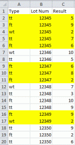
As an example, the figure below would be the result before filtering:

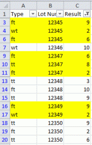
and the next figure would be the result after filtering (5 & 7 filtered from result column):

I hope that this provides another useful bullet to your Excel formatting arsenal.